1 Free Constructions and Comma Categories
1.1 Setting up the Problem
Discussion 1.1.1. The first part of this book is concerned with constructing universal objects of various sorts. These objects will be constructed following a common pattern, which we will first witness here. These constructions all have a local and a global flavor. This chapter focuses on two simple, local cases, the free vector space on a set and the free algebra on a set. These problems are local insofar as they are concerned with a construction for a single, particular set \(X\). The next chapter will be global in that it will consider what happens when we take all the particular solutions and try to assemble them into a single, global construction. Ultimately, we care about getting to the geometric algebra construction, which starts from the tensor algebra. The tensor algebra itself starts from the free algebra on a set, which is the main focus here.
Fix a set \(X\). What should it mean to construct a vector space (or an algebra) out of \(X\)? By itself \(X\) only has set structure. We can see what its elements are, take subsets, etc. We cannot add elements or scale them as in a vector space or multiply them as in an algebra. Among the many ways to make \(X\) into a vector space or an algebra, is there an optimal one? What would “optimal” mean here?
Focus on the vector space problem first. Fix a field \(K\) and pick any vector space \(V \in \mathsf{Vect}_K\) (the \(\in\) is informal: the vector spaces over \(K\) do not form a set). Now \(X \in \mathsf{Set}\) and \(V \in \mathsf{Vect}_K\). We can imagine looking at maps \(X \xrightarrow{f} V\). Since \(V\) is a vector space, we can view the combination of \(V\) and \(X \xrightarrow{f} V\) as a way to equip \(X\) with a vector space structure. This is a loose way of speaking: \(f\) need not be injective and its image need not be a subspace, so no vector space structure is placed on \(X\) itself. What we are really after is a mapping of \(X\) into a vector space. We will keep saying “make \(X\) into a vector space” informally in discussion, but precise statements will always speak of maps.
There is a minor but circumventable problem, however. \(X\) and \(V\) are in different categories. We need some common category to have an arrow. But every vector space \(V\) is really a triple \((V, +, \cdot)\), where \(V\) is the set, \(+\) the vector addition, and \(\cdot\) the scalar multiplication. (Here \(V\) is doing double duty, naming both the vector space and its set of vectors; the functor below separates the two.) Every vector space already has a set, so \(f\) can just be a regular function. In fact, we have a functor 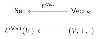 which maps every vector space to its set of vectors.
So, for our fixed set \(X \in \mathsf{Set}\), we care about pairs of a vector space \(V\) and a function \(X \xrightarrow{f} U^{\mathsf{Vect}}_{}(V)\). The following example shows how much the function matters, even with the vector space fixed.
Example 1.1.2. Take the two-element set \(X = \{a, b\}\) and the vector space \(V = \mathbb{R}^2\) with the standard basis \(e_1 = (1, 0)\) and \(e_2 = (0, 1)\). Consider the maps 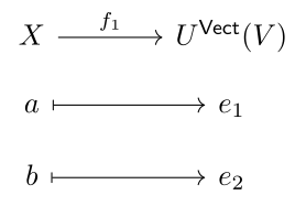 and
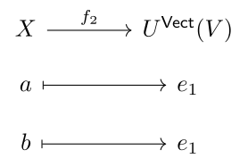 These maps give different ways to make \(X\) into a vector space, with the image of \(f_1\) spanning all of \(\mathbb{R}^2\) while \(f_2\) identifies \(a\) and \(b\).
Discussion 1.1.3. So we care about pairs \((V, X \xrightarrow{f} U^{\mathsf{Vect}}_{}(V))\) for \(V \in \mathsf{Vect}_K\) and \(f \in \mathsf{Set}(X, U^{\mathsf{Vect}}_{}(V))\). In general, for a category \(\mathsf{C}\), we write \(\mathsf{C}(x, y)\) for the set of arrows \(x \to y\) in \(\mathsf{C}\); many algebra texts write \(\mathop{\mathrm{Hom}}_{\mathsf{C}}(x, y)\). So \(\mathsf{Set}(X, U^{\mathsf{Vect}}_{}(V))\) is the set of functions \(X \to U^{\mathsf{Vect}}_{}(V)\).
That is progress, although we still have no criterion for what would constitute an optimal pair. In order to answer that, we need some way of relating a pair \((V_1, X \xrightarrow{f_1} U^{\mathsf{Vect}}_{}(V_1))\) to some other pair \((V_2, X \xrightarrow{f_2} U^{\mathsf{Vect}}_{}(V_2))\).
If we seek to relate pairs, does that mean we want things like  that is, do we want to make a category whose objects are our pairs \((V, f)\) and whose arrows are still to be determined? And, if we can build such a category, could the optimal solution be an initial or terminal object in our category of solutions?
The next section builds that category and shows why in our two cases (making a set into a vector space or an algebra), the universal solution should be an initial object.
Exercises
Exercise 1.1.1. Let \(X = \{a, b\}\) and \(V = \mathbb{R}^2\).
Describe all functions \(f\colon X \to U^{\mathsf{Vect}}_{}(\mathbb{R}^2)\) for which \(f(a)\) and \(f(b)\) span \(\mathbb{R}^2\).
Describe all those for which \(f(a)\) and \(f(b)\) span a line or less.
Which of the pairs \((\mathbb{R}^2, f)\) lose information about \(X\), and in what sense?
Exercise 1.1.2. Let \(f\colon X \to U^{\mathsf{Vect}}_{}(V)\) be a function, let \[W \coloneqq \operatorname{span}(f(X)) \subseteq V,\] and write \(\iota\colon W \hookrightarrow V\) for the inclusion.
Show that there is a function \(f'\colon X \to U^{\mathsf{Vect}}_{}(W)\) with \(f = U^{\mathsf{Vect}}_{}(\iota) \circ f'\).
In what sense is the pair \((W, f')\) “smaller” than \((V, f)\)?
How does \(\iota\) relate the pairs \((W, f')\) and \((V, f)\)?
1.2 Comma Categories and Free Objects
Discussion 1.2.1. Before getting to our specific situation, let us step back to introduce the general construction of comma categories. In comma categories we have two categories \(\mathsf{A}\) and \(\mathsf{B}\) that we want to compare. We need some common place to compare them, which is some ambient category \(\mathsf{C}\). We need some way of getting \(\mathsf{A}\) and \(\mathsf{B}\) into \(\mathsf{C}\), so we do not just have \(\mathsf{A}\), but also a functor \(\mathsf{A} \xrightarrow{S} \mathsf{C}\). Likewise we also have a functor \(\mathsf{B} \xrightarrow{T} \mathsf{C}\). Our comparisons in \(\mathsf{C}\) depend not just on \(\mathsf{A}\) and \(\mathsf{B}\), but also on how \(\mathsf{A}\) and \(\mathsf{B}\) map into \(\mathsf{C}\). We have the following diagram 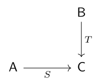
We want to build a category from this data. Given our motivation of comparing \(\mathsf{A}\) to \(\mathsf{B}\) inside \(\mathsf{C}\) it is reasonable to take our objects as triples, an object \(a\) from \(\mathsf{A}\), an object \(b\) from \(\mathsf{B}\), and a comparison in \(\mathsf{C}\) which is an arrow \(f \in \mathsf{C}(S(a), T(b))\).
Given our objects are triples \((a, b, S(a) \xrightarrow{f} T(b))\) what are our arrows? Say we have objects \((a_1, b_1, S(a_1) \xrightarrow{f_1} T(b_1))\) and \((a_2, b_2, S(a_2) \xrightarrow{f_2} T(b_2))\), a map from one to the other should include an arrow \(a_1 \xrightarrow{h} a_2\), i.e. \(h \in \mathsf{A}(a_1, a_2)\). It should also include \(b_1 \xrightarrow{k} b_2\), i.e. \(k \in \mathsf{B}(b_1, b_2)\). But these maps should also coherently map  That is relatively simple, given that the functor \(S\) maps
 and \(T\) maps

Putting this together we define an arrow to be a pair \((h, k)\) 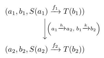 such that
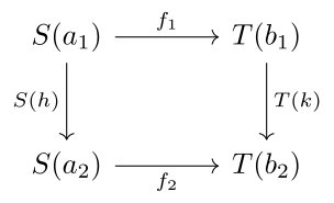 commutes (\(h\) and \(k\) need to map the arrow \(f_1\) to the arrow \(f_2\) via \(S(h)\) and \(T(k)\)). We gather this all together as a definition.
Definition 1.2.2. Fix where \(\mathsf{A}\), \(\mathsf{B}\) and \(\mathsf{C}\) are categories and \(S\) and \(T\) functors. The comma category \(S \downarrow T\) has
objects: triples \((a, b, S(a) \xrightarrow{f} T(b))\) for \(a \in \mathsf{A}\), \(b \in \mathsf{B}\), and \(f \in \mathsf{C}(S(a), T(b))\);
arrows: pairs \((a_1, b_1, f_1) \xrightarrow{(h, k)} (a_2, b_2, f_2)\) with \(h \in \mathsf{A}(a_1, a_2)\) and \(k \in \mathsf{B}(b_1, b_2)\) such that
commutes.
Composition is componentwise, \((h', k') \circ (h, k) \coloneqq (h' \circ h, k' \circ k)\), and the identity on \((a, b, f)\) is \((1_a, 1_b)\). Exercise 1.2.1 checks that these are arrows of \(S \downarrow T\) and that \(S \downarrow T\) is a category.
Discussion 1.2.3. Having defined comma categories in general, let us now specialize to the cases of interest to us. Fix a set \(X\). We are concerned with ways to make \(X\) into a vector space and into an algebra. For the vector space problem we are interested in pairs \((V, X \xrightarrow{f} U^{\mathsf{Vect}}_{}(V))\), where \(V\) is a vector space and \(f\) is a function from \(X\) to \(V\), regarded as a set. For the algebra problem we are concerned with pairs \((A, X \xrightarrow{f} U^{\mathsf{Alg}}_{}(A))\) where \(A\) is an algebra and \(f\) a function from \(X\) to \(A\), regarded as a set. Vector spaces and fields we take as known. Algebras we define now, since this is their first real use.
Definition 1.2.4. A (unital, associative) \(K\)-algebra is a vector space \(A\) over a field \(K\) together with a multiplication function \[\otimes\colon A \times A \to A\] and an element \(1_\otimes \in A\) (written \(1_A\) when we need to say which algebra) such that, for all \(a, b, c \in A\) and \(\lambda \in K\),
\(\otimes\) is bilinear: it is linear in each argument separately, \[\begin{align*} (a + b) \otimes c &= a \otimes c + b \otimes c, & (\lambda a) \otimes c &= \lambda (a \otimes c), \\ a \otimes (b + c) &= a \otimes b + a \otimes c, & a \otimes (\lambda c) &= \lambda (a \otimes c); \end{align*}\]
\(\otimes\) is associative: \((a \otimes b) \otimes c = a \otimes (b \otimes c)\);
\(1_\otimes\) is a unit: \(1_\otimes \otimes a = a = a \otimes 1_\otimes\).
The left column of the bilinearity conditions is the two distributive laws; the right column says scalars can be moved in and out of either factor. The algebra is commutative if moreover \(a \otimes b = b \otimes a\) for all \(a, b \in A\). We do not assume algebras are commutative.
Remark 1.2.5. In the literature “algebra” often means only a vector space with a bilinear multiplication, and the two further axioms are optional. Lie algebras are the classic case: the bracket \([a, b]\) is neither associative nor unital, and satisfies the Jacobi identity instead. Associative algebras without a unit are common too; the finitely supported functions under pointwise multiplication are one (Exercise 1.2.5). In this book every algebra is unital and associative, because the tensor, exterior and geometric algebras all are. Lie algebras will still make an appearance later, inside a geometric algebra, as the bivectors under the commutator.
Commutativity is a different kind of dividing line. Commutative algebras behave like rings of functions on a space (polynomials, continuous functions), and much of algebraic geometry is the study of that correspondence; non-commutative algebras behave like rings of operators (matrices, differential operators), and their elements record order. The free algebra on a set is as non-commutative as an algebra can be, and the geometric algebras we are heading for inherit that: in them \(ab\) and \(ba\) carry different geometric information. The next chapter builds the commutative counterpart of the free algebra too, the symmetric algebra, and the contrast between the two is instructive.
Definition 1.2.6. The category \(\mathsf{Alg}_K\) has as objects the \(K\)-algebras and as arrows the algebra homomorphisms, where an algebra homomorphism \((A, \otimes, 1_\otimes) \to (A', \otimes', 1_{\otimes'})\) is a linear map \(g\colon A \to A'\) with \[g(a \otimes b) = g(a) \otimes' g(b) \quad\text{and}\quad g(1_\otimes) = 1_{\otimes'}\] for all \(a, b \in A\). Composition and identities are those of linear maps (Exercise 1.2.3 checks that these are homomorphisms). The functor \(U^{\mathsf{Alg}}_{}\colon \mathsf{Alg}_K \to \mathsf{Set}\) sends an algebra to its underlying set and a homomorphism to itself, regarded as a function.
Remark 1.2.7. There is usually only one addition in sight, but there are often several multiplications: the field’s, the algebra’s, and later the products of tensor and geometric algebras. In many texts each is written by juxtaposition, and the reader is left to work out which product \(ab\) means. Until the end of this chapter we write a generic algebra or monoid product as \(\otimes\), so that it can be told apart from the field’s multiplication and from juxtaposition. In the future chapters \(\otimes\) is reserved for one specific product, the tensor product, and the generic product gets its own treatment there.
Example 1.2.8. Three \(K\)-algebras, each with its own flavor.
The field \(K\) itself, as a one-dimensional vector space over \(K\), with its own multiplication and unit \(1\). Bilinearity is just the field axioms. It is commutative, and it is the smallest algebra with \(1 \neq 0\) (Exercise 1.2.4 shows it is initial in \(\mathsf{Alg}_K\)).
The polynomials \(K[t]\) in one variable, with the usual product and unit the constant polynomial \(1\). It is commutative and infinite-dimensional, with basis \(1, t, t^2, \ldots\). Every element is a finite linear combination of powers of the single element \(t\); the free algebra on a one-element set will turn out to be exactly this (Example 1.5.19).
The \(n \times n\) matrices \(\mathrm{M}_n(K)\), with matrix multiplication and unit the identity matrix \(I\). For \(n \geq 2\) it is not commutative: already \(\bigl(\begin{smallmatrix} 0 & 1 \\ 0 & 0 \end{smallmatrix}\bigr) \bigl(\begin{smallmatrix} 0 & 0 \\ 1 & 0 \end{smallmatrix}\bigr) \neq \bigl(\begin{smallmatrix} 0 & 0 \\ 1 & 0 \end{smallmatrix}\bigr) \bigl(\begin{smallmatrix} 0 & 1 \\ 0 & 0 \end{smallmatrix}\bigr)\). Nothing in Definition 1.2.4 asks for commutativity, and the algebras this book is heading for are, like \(\mathrm{M}_n(K)\), not commutative.
Discussion 1.2.9. Here and throughout, algebra means unital associative \(K\)-algebra. Our goal is to show how our problems are special cases of the comma category construction. A general object in \(S \downarrow T\) is \((a, b, S(a) \xrightarrow{f} T(b))\). Focusing on the vector space problem for a moment, we have a pair \((V, X \xrightarrow{f} U^{\mathsf{Vect}}_{}(V))\). This makes clear that we have \(? \downarrow U^{\mathsf{Vect}}_{}\) as in 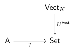 All that remains is to figure out \(\mathsf{A}\) and \(\mathsf{A} \xrightarrow{?} \mathsf{Set}\). We need the functor to pick out the set \(X\), so we let \(\mathsf{A}\) be the terminal category \(\mathsf{1}\) (one object with the only arrow the identity morphism on that object) and the functor should be \(\mathsf{1}\xrightarrow{X} \mathsf{Set}\) that maps the single object in \(\mathsf{1}\) to \(X\) and identity morphism to \(1_X\). We also write \(X\) for this functor \(\mathsf{1}\to \mathsf{Set}\); context makes clear whether \(X\) means the set or the functor.
With this in hand we have recast our two problems in categorical terms. For the vector space problem of how to make a set into a vector space we care about the comma category \(X \downarrow U^{\mathsf{Vect}}_{}\) as in the diagram 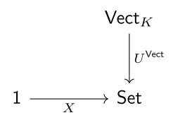 For the algebra problem we care about \(X \downarrow U^{\mathsf{Alg}}_{}\) as in
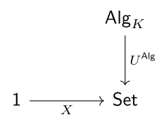
Strictly, an object of \(X \downarrow U^{\mathsf{Vect}}_{}\) is a triple \((\ast, V, f)\), where \(\ast\) is the single object of \(\mathsf{1}\), and an arrow \((\ast, V, f) \to (\ast, V', f')\) is a pair \((1_\ast, g)\) with \(g\colon V \to V'\) linear and \(U^{\mathsf{Vect}}_{}(g) \circ f = f'\). The entries coming from \(\mathsf{1}\) carry no information, so we drop them: we write objects as pairs \((V, f)\) and arrows as linear maps \(g\) with \(U^{\mathsf{Vect}}_{}(g) \circ f = f'\). The same goes for \(X \downarrow U^{\mathsf{Alg}}_{}\).
From here on the algebra problem runs exactly parallel to the vector space problem: replace \(\mathsf{Vect}_K\), \(U^{\mathsf{Vect}}_{}\), vector spaces and linear maps by \(\mathsf{Alg}_K\), \(U^{\mathsf{Alg}}_{}\), algebras and algebra homomorphisms. We will still state the algebra versions of definitions and results in full. Readers comfortable with the pattern may find this repetitive; we accept that so that every statement is on the page rather than left to the reader to translate.
Sticking with the vector space problem, what have we gained by framing it in terms of \(X \downarrow U^{\mathsf{Vect}}_{}\)?
Every object in \(X \downarrow U^{\mathsf{Vect}}_{}\) is a pair \((V, X \xrightarrow{f} U^{\mathsf{Vect}}_{}(V))\). This object is a particular way to make \(X\) into a vector space. Making this a category means solutions do not live in isolation. Arrows in \(X \downarrow U^{\mathsf{Vect}}_{}\) are ways to map one solution to another. This gives a potential candidate for what an optimal solution to our problems could be.
Heuristic. A good first guess, when a category is in play and we want some distinguished object, is an initial or terminal object.
Given that the objects in our category are solutions to a particular problem, an initial or terminal object would mean that every particular solution is related to the initial or terminal object in a unique way. In our cases, the terminal objects will be trivial in a way that carries no information.
So our task now is to determine whether an initial or a terminal object in \(X \downarrow U^{\mathsf{Vect}}_{}\) (respectively, \(X \downarrow U^{\mathsf{Alg}}_{}\)) is the right notion of a universal way to map \(X\) to a vector space (resp. an algebra).
Proposition 1.2.10. The object \((\mathbf{0}, X \xrightarrow{!} U^{\mathsf{Vect}}_{}(\mathbf{0}))\), where \(\mathbf{0}\) is the zero vector space and \(!\) the unique function into its one-point set, is terminal in \(X \downarrow U^{\mathsf{Vect}}_{}\). Likewise the zero algebra, with the unique function from \(X\), is terminal in \(X \downarrow U^{\mathsf{Alg}}_{}\).
Sketch 1.2.11 (of Proposition 1.2.10). The category \(\mathsf{Vect}_K\) has a zero object (an object that is initial and terminal), namely the vector space with the single element \(0\). Writing \(\mathbf{0}\) for this vector space, one shows that \((\mathbf{0}, X \xrightarrow{!} U^{\mathsf{Vect}}_{}(\mathbf{0}))\) is terminal in \(X \downarrow U^{\mathsf{Vect}}_{}\) (Exercise 1.2.7). It is also easy to see that, unless \(X = \varnothing\), \((\mathbf{0}, X \xrightarrow{!} U^{\mathsf{Vect}}_{}(\mathbf{0}))\) is not initial in \(X \downarrow U^{\mathsf{Vect}}_{}\) (Exercise 1.2.8). The same facts hold for \(X \downarrow U^{\mathsf{Alg}}_{}\) (Exercise 1.2.9).
Discussion 1.2.12. So terminal objects in \(X \downarrow U^{\mathsf{Vect}}_{}\) and \(X \downarrow U^{\mathsf{Alg}}_{}\) are not interesting. Are initial objects? If we had an initial object \(\mathbf{0}_{X \downarrow U^{\mathsf{Vect}}_{}}\), what would that give? We will write such an object as \(\mathbf{0}_{X \downarrow U^{\mathsf{Vect}}_{}} = (F^{}_{\mathsf{Vect}}(X), X \xrightarrow{\eta^{\mathsf{Vect}}_{X}} U^{\mathsf{Vect}}_{}(F^{}_{\mathsf{Vect}}(X)))\).
If we have such a pair then for any other solution \((V, X \xrightarrow{f} U^{\mathsf{Vect}}_{}(V))\) we have 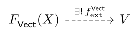 such that
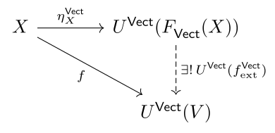 commutes.
Take a moment with this. If we have the single solution \[\mathbf{0}_{X \downarrow U^{\mathsf{Vect}}_{}} = (F^{}_{\mathsf{Vect}}(X), X \xrightarrow{\eta^{\mathsf{Vect}}_{X}} U^{\mathsf{Vect}}_{}(F^{}_{\mathsf{Vect}}(X))),\] then any other solution \((V, X \xrightarrow{f} U^{\mathsf{Vect}}_{}(V))\) is derived from the initial solution by the unique (forced) arrow \[F^{}_{\mathsf{Vect}}(X) \xrightarrow{f^{\mathsf{Vect}}_{\mathrm{ext}}} V.\]
Heuristic. \(\mathbf{0}_{X \downarrow U^{\mathsf{Vect}}_{}}\) carries every other solution’s information inside it in the most compact fashion.
This is a fitting characterization of a universal solution to our problem. We can now restate our problems rigorously as definitions: first the vector space problem, then the algebra problem.
Definition 1.2.13. Let \(X\) be a set. A free vector space on \(X\) is an initial object \[(F^{}_{\mathsf{Vect}}(X), X \xrightarrow{\eta^{\mathsf{Vect}}_{X}} U^{\mathsf{Vect}}_{}(F^{}_{\mathsf{Vect}}(X)))\] of \(X \downarrow U^{\mathsf{Vect}}_{}\).
That is, for every vector space \(V\) and function \(f\colon X \to U^{\mathsf{Vect}}_{}(V)\) there is exactly one linear map \[F^{}_{\mathsf{Vect}}(X) \xrightarrow{f^{\mathsf{Vect}}_{\mathrm{ext}}} V\] such that commutes.
We call \(\eta^{\mathsf{Vect}}_{X}\) the unit map (it depends on both the set \(X\) and the functor \(U^{\mathsf{Vect}}_{}\), which its subscript and superscript record) and \(f^{\mathsf{Vect}}_{\mathrm{ext}}\) the extension of \(f\).
Definition 1.2.14. Let \(X\) be a set. A free algebra on \(X\) is an initial object \[(F^{}_{\mathsf{Alg}}(X), X \xrightarrow{\eta^{\mathsf{Alg}}_{X}} U^{\mathsf{Alg}}_{}(F^{}_{\mathsf{Alg}}(X)))\] of \(X \downarrow U^{\mathsf{Alg}}_{}\).
That is, for every \(K\)-algebra \(A\) and function \(f\colon X \to U^{\mathsf{Alg}}_{}(A)\) there is exactly one algebra homomorphism \[F^{}_{\mathsf{Alg}}(X) \xrightarrow{f^{\mathsf{Alg}}_{\mathrm{ext}}} A\] such that 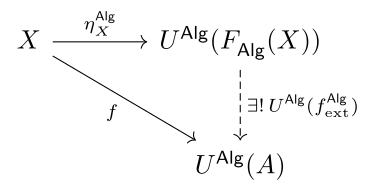 commutes.
We call \(\eta^{\mathsf{Alg}}_{X}\) the unit map (it depends on both the set \(X\) and the functor \(U^{\mathsf{Alg}}_{}\)) and \(f^{\mathsf{Alg}}_{\mathrm{ext}}\) the extension of \(f\).
Discussion 1.2.15. A few remarks. Definition 1.2.14 is Definition 1.2.13 with \(\mathsf{Alg}_K\) and \(U^{\mathsf{Alg}}_{}\) in place of \(\mathsf{Vect}_K\) and \(U^{\mathsf{Vect}}_{}\).
Crucially, any two free vector spaces on \(X\) are related by a unique isomorphism compatible with their unit maps, that is, a unique isomorphism in \(X \downarrow U^{\mathsf{Vect}}_{}\) (Exercise 1.2.10). So we speak of the free vector space on \(X\). The same holds for free algebras, allowing us to speak of the free algebra on \(X\).
Finally, to this point we have worked just to state our problems well. Now we need to see if they have solutions. There is no a priori reason that a given set \(X\) has either a free vector space or a free algebra. If none existed, the definitions would describe nothing. The next three sections show each problem does, in fact, have a universal solution for every set \(X\).
Exercises
Exercise 1.2.1. Let \(S\colon \mathsf{A} \to \mathsf{C}\) and \(T\colon \mathsf{B} \to \mathsf{C}\) be functors.
Composition. For arrows \[(a_1, b_1, f_1) \xrightarrow{(h, k)} (a_2, b_2, f_2) \xrightarrow{(h', k')} (a_3, b_3, f_3)\] of \(S \downarrow T\), show that the composite \((h', k') \circ (h, k) = (h' \circ h, k' \circ k)\) is again an arrow of \(S \downarrow T\).
Identities. For an object \((a, b, f)\), show that \((1_a, 1_b)\) is an arrow \((a, b, f) \to (a, b, f)\).
Show that with this composition and these identities, \(S \downarrow T\) is a category: composition is associative and the \((1_a, 1_b)\) are two-sided units.
Exercise 1.2.2. For an object \(c\) of \(\mathsf{C}\), write \(c\colon \mathsf{1}\to \mathsf{C}\) for the functor picking out \(c\), and \(1_{\mathsf{C}}\) for the identity functor.
Show that \(1_{\mathsf{C}} \downarrow c\) is the category of objects over \(c\) (the slice) and \(c \downarrow 1_{\mathsf{C}}\) the category of objects under \(c\) (the coslice).
How does \(X \downarrow U^{\mathsf{Vect}}_{}\) differ from a coslice?
Exercise 1.2.3. Show that the composite of two algebra homomorphisms is an algebra homomorphism, and that the identity map of an algebra is one. Conclude that \(\mathsf{Alg}_K\) is a category.
Exercise 1.2.4. Unlike \(\mathsf{Vect}_K\), the category \(\mathsf{Alg}_K\) has no zero object.
Show that \(K\), with its own multiplication and unit \(1\), is a \(K\)-algebra, and that for every algebra \(A\) there is exactly one algebra homomorphism \(K \to A\). So \(K\) is initial in \(\mathsf{Alg}_K\).
Show that the zero vector space \(\mathbf{0}\), with its only possible multiplication and \(1_\otimes = 0\), is a \(K\)-algebra (the zero algebra), and that it is terminal in \(\mathsf{Alg}_K\).
Show that \(K\) and the zero algebra are not isomorphic, so that \(\mathsf{Alg}_K\) has no object that is both initial and terminal. Where does the argument that \(\mathbf{0}\) is initial in \(\mathsf{Vect}_K\) break down for algebras?
Exercise 1.2.5. Decide which of the following make the given vector space into a \(K\)-algebra, and for each failure name the axiom that fails.
\(\mathbb{R}^2\) with componentwise multiplication \((a_1, a_2) \otimes (b_1, b_2) \coloneqq (a_1 b_1, a_2 b_2)\).
\(\mathbb{R}^3\) with the cross product \(a \otimes b \coloneqq a \times b\).
\(\mathbb{R}\) with \(a \otimes b \coloneqq a + b\).
\(\mathbb{R}^2\) with \((a_1, a_2) \otimes (b_1, b_2) \coloneqq (a_1 b_1, 0)\).
The space \(K^X\) of Notation 1.3.2, with pointwise multiplication \((\phi \otimes \psi)(x) \coloneqq \phi(x)\psi(x)\).
Exercise 1.2.6. Let \(A\) be a \(K\)-algebra. Write \(u\colon K \to A\) for the linear map \(\lambda \mapsto \lambda\, 1_\otimes\), and \(\cdot\) for scalar multiplication.
Show that associativity of \(\otimes\) says exactly that
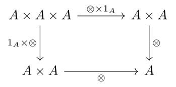 commutes in \(\mathsf{Set}\).
Show that the unit laws say exactly that
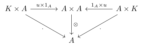 commutes.
Try to express bilinearity as the commutativity of a diagram in \(\mathsf{Set}\) or in \(\mathsf{Vect}_K\) in the same style. What goes wrong?
Exercise 1.2.7. Show that \((\mathbf{0}, X \xrightarrow{!} U^{\mathsf{Vect}}_{}(\mathbf{0}))\), where \(\mathbf{0}\) is the single-element vector space (consisting only of \(0\)) and \(!\) is the unique function into the one-point set \(U^{\mathsf{Vect}}_{}(\mathbf{0})\), is terminal in \(X \downarrow U^{\mathsf{Vect}}_{}\).
Exercise 1.2.8. Consider the object \((\mathbf{0}, X \to U^{\mathsf{Vect}}_{}(\mathbf{0}))\) of \(X \downarrow U^{\mathsf{Vect}}_{}\).
Show that if \(X \neq \varnothing\), then it is not initial.
Show that if \(X = \varnothing\), then it is initial. What does this say about the free vector space on \(\varnothing\)?
Exercise 1.2.9. State and prove the analogues of Exercises 1.2.7 and 1.2.8 for \(X \downarrow U^{\mathsf{Alg}}_{}\), using the zero algebra (the algebra in which \(1 = 0\)). Is the zero algebra initial in \(\varnothing \downarrow U^{\mathsf{Alg}}_{}\)?
Exercise 1.2.10. Let \(a\) and \(a'\) be initial objects of a category \(\mathsf{C}\).
Show that there is exactly one isomorphism \(a \to a'\) in \(\mathsf{C}\).
Deduce that any two free vector spaces on \(X\) are related by a unique isomorphism compatible with their unit maps, and likewise for free algebras. (This is what entitles us to speak of the free vector space and the free algebra.)
1.3 Constructing Free Vector Spaces
Discussion 1.3.1. Our task in this section is to construct a free vector space on an arbitrary set \(X\). First, we construct a viable candidate. Remember that what we are actually choosing is a candidate pair: a vector space \(V\) together with a map \(X \to U^{\mathsf{Vect}}_{}(V)\). Equipped with a candidate solution, we prove it is initial in the comma category \(X \downarrow U^{\mathsf{Vect}}_{}\), which makes it a free vector space on \(X\).
We want to map \(X\) into a vector space over \(K\) in the best possible way. So far the only structure in play is that of \(X\), which has none beyond being a set, and that of the field \(K\). We know nothing a priori about what vector space \(V\) we want. An important observation is that the structure our unknown \(V\) must have, vector addition and scalar multiplication, already exists on the field \(K\). Two guiding ideas suggest how to proceed.
Heuristic. To build something with more structure out of a bare set, look at functions defined on the set.
Heuristic. When the structure we want already lives somewhere, map into that place and let it do the work.
Combining the two ideas, we look at functions \(X \to K\).
Notation 1.3.2. For a set \(X\), we write \(K^X\) for the set of all functions \(X \to K\). With the pointwise operations \[\begin{align*} (\lambda\phi)(x) &\coloneqq \lambda\, \phi(x), \\ (\phi + \psi)(x) &\coloneqq \phi(x) + \psi(x), \end{align*}\] for \(\lambda \in K\) and \(\phi, \psi \in K^X\), it is a vector space over \(K\): each axiom holds at every point because it holds in \(K\). Its zero is the function \(x \mapsto 0\).
As a set, \(K^X\) is the hom-set \(\mathsf{Set}(X, K)\); the two notations name the same functions. We write \(K^X\) when we mean this set with its pointwise structure, and \(\mathsf{Set}(X, Y)\) when we mean a bare set of functions, as in Definition 1.4.9.
Discussion 1.3.3. Next we need a function from \(X\) into \(K^X\), sending each \(x \in X\) to some \(\delta_x \in K^X\). Nothing singles out a point of \(X\) except the point \(x\) itself. Helpfully, \(K\) has two distinguished elements that need no choosing, \(0\) and \(1\).
Heuristic. A universal construction should be built only from what the data hands us, with no arbitrary choices. (This is intuition, not a theorem: what we will actually prove is initiality.)
The only choice-free options that single out \(x\) are to map \(x\) to one of \(0\) or \(1\) and every other point to the other. (The constant functions \(0\) and \(1\) are choice-free too, but they do not tell the points of \(X\) apart.) Exercise 1.3.1 shows what goes wrong with the second option. We let \(\delta_x\) be \(1\) at \(x\) and \(0\) elsewhere: \[\begin{array}{rcl} X & \xrightarrow{\delta_x} & K \\ x & \mapsto & 1 \\ y & \mapsto & 0 \quad (y \neq x). \end{array}\] This gives the map \[\begin{array}{rcl} X & \xrightarrow{\delta} & U^{\mathsf{Vect}}_{}(K^X) \\ x & \mapsto & \delta_x, \end{array}\] and our candidate solution is \((K^X, \delta)\). (We will shortly shrink its codomain, and only then give it the tag \(\delta^{\mathsf{Vect}}_X\).)
Let us test our candidate against the universal property, using an arbitrary solution \((V, f\colon X \to U^{\mathsf{Vect}}_{}(V))\). The map \(f\) is just a function, but any extension \(f^{\mathrm{cand}}_{\mathrm{ext}}\colon K^X \to V\) of it must be linear and must satisfy \(f^{\mathrm{cand}}_{\mathrm{ext}}(\delta_x) = f(x)\) (this being the equation form of the commutative triangle for \(f^{\mathrm{cand}}_{\mathrm{ext}}\)).
We know \(f^{\mathrm{cand}}_{\mathrm{ext}}\) on \(\{ \delta_x \}_x \subseteq K^X\). In fact, because \(f^{\mathrm{cand}}_{\mathrm{ext}}\) is linear, we actually know the value of \(f^{\mathrm{cand}}_{\mathrm{ext}}\) on all linear combinations of the \(\delta_x\), since \[\begin{array}{rcl} f^{\mathrm{cand}}_{\mathrm{ext}}\bigl(\sum_{j=1}^n \lambda_j \delta_{x_j}\bigr) & = & \sum_{j=1}^n \lambda_j f^{\mathrm{cand}}_{\mathrm{ext}}(\delta_{x_j}) \\ & = & \sum_{j=1}^n \lambda_j f(x_j). \end{array}\] Our heuristic says we must make no arbitrary choices in a universal construction, and the universal property pins down the value of \(f^{\mathrm{cand}}_{\mathrm{ext}}\) only on the subspace of \(K^X\) generated by the \(\delta_x\). Off that subspace, the value of an extension is a free choice, so we cannot expect it to be unique (Exercise 1.3.2). It stands to reason that instead of taking all of \(K^X\) as our domain, we should consider only the subspace generated by the \(\delta_x\), which is the set of their finite linear combinations: \[\operatorname{span}\{\delta_x \mid x \in X\} = \Bigl\{\, \sum_{j=1}^n \lambda_j \delta_{x_j} \Bigm| n \in \mathbb{N},\ \lambda_j \in K,\ x_1, \ldots, x_n \in X \text{ distinct} \,\Bigr\}.\] The key is that this span consists of finite sums, so any function in the span of the \(\delta_x\) is nonzero on only finitely many inputs. This is not an issue if the set \(X\) is finite. If, however, \(X\) is an infinite set, then an arbitrary \(\phi \in K^X\) can have infinitely many inputs with non-zero outputs. This motivates the following definitions.
Definition 1.3.4. For a function \(X \xrightarrow{\phi} K\) where \(X\) is a set and \(K\) is a field, \[\mathop{\mathrm{supp}}(\phi) \coloneqq \{\, x \in X \mid \phi(x) \neq 0 \,\}.\]
Definition 1.3.5. A function \(\phi\colon X \to K\) is finitely supported if \(\mathop{\mathrm{supp}}(\phi)\) is finite. We write \[K^{(X)} \coloneqq \{\, \phi \in K^X \mid \mathop{\mathrm{supp}}(\phi) \text{ is finite} \,\}.\]
Lemma 1.3.6. \(K^{(X)}\) is a subspace of \(K^X\). In particular, it is a vector space under the pointwise operations.
Proof 1.3.7 (of Lemma 1.3.6). The zero function has empty support. For \(\lambda \in K\) and \(\phi, \psi \in K^{(X)}\), \[\mathop{\mathrm{supp}}(\lambda\phi) \subseteq \mathop{\mathrm{supp}}(\phi) \quad\text{and}\quad \mathop{\mathrm{supp}}(\phi + \psi) \subseteq \mathop{\mathrm{supp}}(\phi) \cup \mathop{\mathrm{supp}}(\psi),\] since if \(\phi(x) = \psi(x) = 0\) then \(\lambda\phi(x) = 0\) and \(\phi(x) + \psi(x) = 0\). A subset of a finite set is finite, and so is a union of two finite sets.
Lemma 1.3.8. \(\{\delta_x \mid x \in X\}\) is a basis for \(K^{(X)}\).
Proof 1.3.9 (of Lemma 1.3.8). We need to show \(\{\delta_x \mid x \in X\}\) is linearly independent and spans \(K^{(X)}\). For linear independence, say \[\lambda_1 \delta_{x_1} + \lambda_2 \delta_{x_2} + \cdots + \lambda_n \delta_{x_n} = 0\] for distinct \(x_1, \ldots, x_n\) and \(\lambda_1, \ldots, \lambda_n \in K\) (\(0\) being the zero function in \(K^{(X)}\)). Let \(\psi \coloneqq \lambda_1 \delta_{x_1} + \cdots + \lambda_n \delta_{x_n} \in K^{(X)}\). \[\begin{align*} \psi(x) &= (\lambda_1 \delta_{x_1} + \cdots + \lambda_n \delta_{x_n})(x) \\ &\coloneqq \lambda_1 \delta_{x_1}(x) + \cdots + \lambda_n \delta_{x_n}(x) \end{align*}\] Now if \(x\) is not one of the \(x_1, \ldots, x_n\), then every \(\delta_{x_j}(x) = 0\), and the sum is \(0_K\). If \(x = x_j\) for one of the \(j\)’s, then the sum becomes \[0 = \lambda_j \delta_{x_j}(x_j) = \lambda_j\] (the other \(\delta_{x_k}(x_j) = 0\)). So all \(\lambda_j = 0\) and we have linear independence.
For spanning, assume \(\phi \in K^{(X)}\). Then \(\mathop{\mathrm{supp}}(\phi)\) is finite. Take \[\phi' \coloneqq \sum_{x \in \mathop{\mathrm{supp}}(\phi)} \phi(x)\, \delta_x(-),\] which, to be clear, is the function \[\Bigl[\sum_{x \in \mathop{\mathrm{supp}}(\phi)} \phi(x)\, \delta_x(-)\Bigr](y) \coloneqq \sum_{x \in \mathop{\mathrm{supp}}(\phi)} \phi(x)\, \delta_x(y).\] Then for \(y \notin \mathop{\mathrm{supp}}(\phi)\), \[\phi'(y) = \sum_{x \in \mathop{\mathrm{supp}}(\phi)} \phi(x)\, \delta_x(y)\] and \(\delta_x(y) = 0\) for every term, making the sum \(0\). If \(y \in \mathop{\mathrm{supp}}(\phi)\) \[\begin{align*} \phi'(y) &= \sum_{x \in \mathop{\mathrm{supp}}(\phi)} \phi(x)\, \delta_x(y) \\ &= \phi(y)\, \delta_y(y) \\ &= \phi(y). \end{align*}\] So \(\phi' = \phi\) and \(\{\delta_x \mid x \in X\}\) spans \(K^{(X)}\).
Each \(\delta_x\) has support \(\{x\}\), so it lies in \(K^{(X)}\). The map \(\delta\) of Discussion 1.3.3 therefore lands in \(K^{(X)}\), and this is the map that gets the tag: \[\begin{array}{rcl} X & \xrightarrow{\delta^{\mathsf{Vect}}_{X}} & U^{\mathsf{Vect}}_{}(K^{(X)}) \\ x & \mapsto & \delta_x. \end{array}\] Our candidate is now \((K^{(X)}, \delta^{\mathsf{Vect}}_X)\).
A word on names. Before we know a candidate is free, a map \(K^{(X)} \to V\) that we hope is the extension of \(f\) is written \(f^{\mathrm{cand}}_{\mathrm{ext}}\); two such maps being compared are \(f^{\mathrm{cand}}_1\) and \(f^{\mathrm{cand}}_2\). The name \(f^{\mathsf{Vect}}_{\mathrm{ext}}\) is reserved for the extension out of a free vector space, and is earned only once initiality is proved.
We can now prove our first significant result.
Theorem 1.3.10. \((K^{(X)}, X \xrightarrow{\delta^{\mathsf{Vect}}_{X}} U^{\mathsf{Vect}}_{}(K^{(X)}))\) is initial in \(X \downarrow U^{\mathsf{Vect}}_{}\); that is, it is a free vector space on \(X\).
Proof 1.3.11 (of Theorem 1.3.10). We need to take an arbitrary object of \(X \downarrow U^{\mathsf{Vect}}_{}\) and show there exists a unique morphism from \((K^{(X)}, X \xrightarrow{\delta^{\mathsf{Vect}}_{X}} U^{\mathsf{Vect}}_{}(K^{(X)}))\) to it. Given \((V, X \xrightarrow{f} U^{\mathsf{Vect}}_{}(V))\), we need 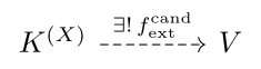 a unique, linear map \(f^{\mathrm{cand}}_{\mathrm{ext}}\) in \(\mathsf{Vect}_K(K^{(X)}, V)\) such that
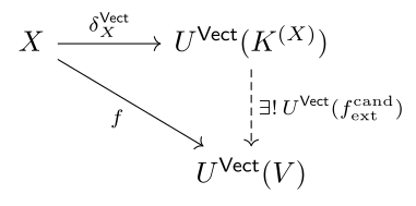 commutes.
How do we construct our linear \(K^{(X)} \xrightarrow{f^{\mathrm{cand}}_{\mathrm{ext}}} V\)? If \(\phi \in K^{(X)}\), \(\phi = \sum_{z \in \mathop{\mathrm{supp}}(\phi)} \phi(z)\, \delta_z(-)\) by the basis lemma just proved. We can map to \(V\) by mapping every \(\delta_z \mapsto f(z) \in U^{\mathsf{Vect}}_{}(V)\) (\(f(z)\) is just a vector). This lets us make our candidate map. \[\begin{array}{rcl} K^{(X)} & \xrightarrow{f^{\mathrm{cand}}_{\mathrm{ext}}} & V \\ \phi = \sum_{z \in \mathop{\mathrm{supp}}(\phi)} \phi(z)\, \delta_z & \mapsto & \sum_{z \in \mathop{\mathrm{supp}}(\phi)} \phi(z)\, f(z) \end{array}\] (Exercise 1.3.3 shows \(f^{\mathrm{cand}}_{\mathrm{ext}}\) is linear)
We need to check that our diagram commutes. \[\begin{array}{rcccl} X & \xrightarrow{\delta^{\mathsf{Vect}}_{X}} & U^{\mathsf{Vect}}_{}(K^{(X)}) & \xrightarrow{U^{\mathsf{Vect}}_{}(f^{\mathrm{cand}}_{\mathrm{ext}})} & U^{\mathsf{Vect}}_{}(V) \\ x & \mapsto & \delta_x = 1_K \cdot \delta_x & \mapsto & 1_K \cdot f(x) = f(x) \end{array}\] and \[\begin{array}{rcl} X & \xrightarrow{f} & U^{\mathsf{Vect}}_{}(V) \\ x & \mapsto & f(x) \end{array}\] so we have that. Finally, is \(f^{\mathrm{cand}}_{\mathrm{ext}}\) unique?
Say \(f^{\mathrm{cand}}_1\) and \(f^{\mathrm{cand}}_2\) both make the triangle commute: \[f(y) = \bigl(U^{\mathsf{Vect}}_{}(f^{\mathrm{cand}}_1) \circ \delta^{\mathsf{Vect}}_{X}\bigr)(y) = \bigl(U^{\mathsf{Vect}}_{}(f^{\mathrm{cand}}_2) \circ \delta^{\mathsf{Vect}}_{X}\bigr)(y).\] Then \[f(y) = U^{\mathsf{Vect}}_{}(f^{\mathrm{cand}}_1)(\delta_y) = U^{\mathsf{Vect}}_{}(f^{\mathrm{cand}}_2)(\delta_y),\] meaning precisely that \[f^{\mathrm{cand}}_1(\delta_y) = f(y) = f^{\mathrm{cand}}_2(\delta_y).\] Since \(f^{\mathrm{cand}}_1\) and \(f^{\mathrm{cand}}_2\) agree on every \(\delta_y\), we then have that \(f^{\mathrm{cand}}_1 = f^{\mathrm{cand}}_2\) (Exercise 1.3.4). So \((K^{(X)}, \delta^{\mathsf{Vect}}_X)\) is a free vector space on \(X\), and from now on we write \(f^{\mathsf{Vect}}_{\mathrm{ext}}\) for \(f^{\mathrm{cand}}_{\mathrm{ext}}\).
Discussion 1.3.12. The proof used only two facts about the \(\delta_x\): an extension of \(f\) must send \(\delta_x\) to \(f(x)\), and the \(\delta_x\) span \(K^{(X)}\). We call the elements of \(X\) (or rather their images \(\delta_x\) under the unit) the generators of the free vector space. The same pattern returns for every free object in this book.
Principle 1.3.13 (Maps out of free objects). A map out of a free object is determined by where it sends the generators, and the generators may be sent anywhere.
The second half is existence of \(f^{\mathsf{Vect}}_{\mathrm{ext}}\): any \(f\) will do. The first half is uniqueness. We will cite this principle for free monoids (§1.4) and free algebras (§1.5).
Example 1.3.14. Let \(X = \{x_1, \ldots, x_n\}\) be finite. Every function \(X \to K\) has finite support, so \(K^{(X)}\) is the space of all functions \(X \to K\), and \[\phi \mapsto (\phi(x_1), \ldots, \phi(x_n))\] is a linear isomorphism \(K^{(X)} \cong K^n\) sending \(\delta_{x_i}\) to the standard basis vector \(e_i\). So the free vector space on an \(n\)-element set is \(K^n\), and its unit sends the \(i\)-th element of \(X\) to \(e_i\).
This revisits Example 1.1.2. With \(X = \{a, b\}\) and \(K = \mathbb{R}\), the map \(f_1\) (\(a \mapsto e_1\), \(b \mapsto e_2\)) is the unit, up to this isomorphism. The map \(f_2\) (\(a, b \mapsto e_1\)) is not initial; it is the composite of the unit with the unique linear extension \(e_1, e_2 \mapsto e_1\). Every other solution factors through the free one in exactly this way.
Exercises
Exercise 1.3.1. Discussion 1.3.3 sends \(x\) to \(1\) and every other point to \(0\). Try it the other way round: for \(x \in X\) let \(\gamma_x \in K^X\) be \(0\) at \(x\) and \(1\) elsewhere, let \(G \subseteq K^X\) be the span of the \(\gamma_x\), and let \(\gamma\colon X \to U^{\mathsf{Vect}}_{}(G)\) send \(x \mapsto \gamma_x\).
Let \(X = \{x\}\) have one element. Show that \(\gamma_x = 0\), and conclude that \((G, \gamma)\) is not a free vector space on \(X\).
Let \(X = \{a, b, c\}\), and let \(K\) be a field in which \(1 + 1 = 0\) (such as \(\mathbb{F}_2\)). Show that \(\gamma_a + \gamma_b + \gamma_c = 0\), and conclude again that \((G, \gamma)\) is not free on \(X\).
Let \(X\) have \(n\) elements, where \(n - 1 \neq 0\) in \(K\). Show that the \(\gamma_x\) form a basis of \(K^X\), and that this time \((G, \gamma)\) is free on \(X\).
So the choice “\(1\) at \(x\)” is not the only one that can work, but it is the only one that works for every set and every field.
Exercise 1.3.2. What goes wrong if we keep all of \(K^X\) (Discussion 1.3.3) when \(X\) is infinite? Take \(X = \mathbb{N}\), so that \(K^{\mathbb{N}}\) is the space of all sequences \((\lambda_0, \lambda_1, \lambda_2, \ldots)\) of scalars, and \(\delta_n\) is the sequence with \(1\) in place \(n\) and \(0\) elsewhere.
A function \(f\colon \mathbb{N} \to U^{\mathsf{Vect}}_{}(V)\) is a sequence of vectors \(v_0, v_1, v_2, \ldots\). Explain why \((\lambda_0, \lambda_1, \ldots) \mapsto \sum_n \lambda_n v_n\) does not define a map \(K^{\mathbb{N}} \to V\).
Show that there is a nonzero linear map \(K^{\mathbb{N}} \to K\) sending every \(\delta_n\) to \(0\). Conclude that \((K^{\mathbb{N}}, n \mapsto \delta_n)\) is not initial in \(\mathbb{N} \downarrow U^{\mathsf{Vect}}_{}\): extensions exist, but they are not unique.
Exercise 1.3.3. Show that the map \(f^{\mathrm{cand}}_{\mathrm{ext}}\colon K^{(X)} \to V\) in the proof of Theorem 1.3.10, \(\sum_z \phi(z)\, \delta_z \mapsto \sum_z \phi(z)\, f(z)\), is linear.
Exercise 1.3.4. Show that two linear maps \(g_1, g_2\colon K^{(X)} \to V\) with \(g_1(\delta_y) = g_2(\delta_y)\) for all \(y \in X\) are equal.
Exercise 1.3.5. Let \(p\colon X \to Y\) be a function. Using only the universal property, show that there is a unique linear map \(K^{(X)} \to K^{(Y)}\) sending \(\delta_x\) to \(\delta_{p(x)}\), and that this assignment respects composition of functions and identities.
1.4 Free Monoid
Discussion 1.4.1. Recall from Definition 1.2.4 that an algebra is a vector space with a bilinear, associative multiplication \(\otimes\) that has a unit \(1_\otimes\). Having solved the free vector space on a set problem, we now turn to the free algebra on a set problem, that is, proving some object initial in the comma category \(X \downarrow U^{\mathsf{Alg}}_{}\). This process is more complex than the free vector space on a set problem. There are a few ways we could slice this, but we will consider an algebra as a \(4\)-tuple at the moment: \[A = (U^{\mathsf{Alg}}_{}(A), \otimes, 1_\otimes, +).\] Here \(U^{\mathsf{Alg}}_{}(A)\) is the set of elements of the algebra, \(\otimes\) is the algebra product, \(1_\otimes\) is the unit of multiplication, and \(+\) stands in for the vector space structure, meaning vector addition, the scalars, and scalar multiplication.
We have just proved the universal way to make a set a vector space. That is, we know how to go \(X \mapsto F^{}_{\mathsf{Vect}}(X) = (U^{\mathsf{Vect}}_{}(F^{}_{\mathsf{Vect}}(X)), +)\) in a universal manner. We do not yet know how to take a set and equip it with a multiplication \(\otimes\) and a multiplicative unit.
If we drop the vector space structure from an algebra (which includes the field of scalars) we are left with \((U^{\mathsf{Alg}}_{}(A), \otimes, 1_\otimes)\). This is precisely a monoid, a set with a multiplication and a multiplicative identity (or, more categorically, a one-object category where the elements are the morphisms).
Definition 1.4.2. A monoid is a set \(M\) together with a multiplication function \[\otimes\colon M \times M \to M\] and an element \(1_\otimes \in M\) (written \(1_M\) when we need to say which monoid) such that, for all \(m, m', m'' \in M\),
\(\otimes\) is associative: \((m \otimes m') \otimes m'' = m \otimes (m' \otimes m'')\);
\(1_\otimes\) is a unit: \(1_\otimes \otimes m = m = m \otimes 1_\otimes\).
We write the monoid as the triple \((M, \otimes, 1_\otimes)\), or simply as \(M\). A monoid is what remains of a \(K\)-algebra (Definition 1.2.4) when the vector space structure, and with it bilinearity, is forgotten.
Definition 1.4.3. The category \(\mathsf{Mon}\) has as objects the monoids and as arrows the monoid homomorphisms, where a monoid homomorphism \((M, \otimes, 1_\otimes) \to (M', \otimes', 1_{\otimes'})\) is a function \(g\colon M \to M'\) with \[g(m \otimes m') = g(m) \otimes' g(m') \quad\text{and}\quad g(1_\otimes) = 1_{\otimes'}\] for all \(m, m' \in M\). Composition and identities are those of functions (Exercise 1.4.1). The functor \(U^{\mathsf{Mon}}_{}\colon \mathsf{Mon}\to \mathsf{Set}\) sends a monoid to its underlying set and a homomorphism to itself, regarded as a function.
Remark 1.4.4. An algebra is a vector space carrying a compatible monoid structure, so there are two routes from a bare set \(X\) to an algebra. The route of this chapter makes \(X\) a monoid first, then adds the vector space structure (§1.5). The other route makes \(X\) a vector space first, \(F^{}_{\mathsf{Vect}}(X)\), and then adjoins a universal multiplication to that vector space: this is the tensor algebra of the next chapter, and it needs the tensor product. Both routes arrive at the free algebra on \(X\); the tensor algebra of \(F^{}_{\mathsf{Vect}}(X)\) comes with the distinguished basis \(\{\delta_x\}\) of generators, while the tensor algebra of a general vector space has no preferred basis, and that is the point of building it. We take the monoid route here because every step can be done with what we have in hand, and compare the two in the next chapter.
The second step of the second route must respect the structure the first step built. Forgetting the vector space structure of \(F^{}_{\mathsf{Vect}}(X)\) and taking the free monoid on its underlying set is not that route: its letters are all the vectors of \(F^{}_{\mathsf{Vect}}(X)\), with no relation between the letter \(v + w\) and the letters \(v\) and \(w\), and the result is a far larger algebra that is not free on \(X\).
Example 1.4.5. Some monoids: the first two are not algebras, whereas the last two are algebras with their vector space structure forgotten.
\((\mathbb{N}, +, 0)\). Addition of natural numbers is associative with unit \(0\). There is no vector space structure in sight, so this is a monoid and nothing more. We will meet it again as the free monoid on a one-element set.
\((\mathbb{N}, \cdot, 1)\). The same set with a different multiplication and a different unit is a different monoid: a monoid is the triple, not the set.
\((\mathrm{M}_n(K), \cdot, I)\), the matrices of Example 1.2.8 with matrix multiplication. Forgetting matrix addition and scalar multiplication leaves a monoid, non-commutative for \(n \geq 2\).
\((K^X, \cdot, \mathbf{1})\), all functions \(X \to K\) under pointwise multiplication, with unit the constant function \(\mathbf{1}\) (Exercise 1.2.5). The finitely supported functions \(K^{(X)}\) are closed under pointwise multiplication, but for infinite \(X\) they do not contain \(\mathbf{1}\), so they form a monoid under \(\cdot\) only when \(X\) is finite.
Definition 1.4.6. Let \(X\) be a set. A free monoid on \(X\) is an initial object \[(F^{}_{\mathsf{Mon}}(X), X \xrightarrow{\eta^{\mathsf{Mon}}_{X}} U^{\mathsf{Mon}}_{}(F^{}_{\mathsf{Mon}}(X)))\] of \(X \downarrow U^{\mathsf{Mon}}_{}\) (\(X\) referring to the same functor \(\mathsf{1}\xrightarrow{X} \mathsf{Set}\) as before).
That is, for every monoid \(M\) and function \(f\colon X \to U^{\mathsf{Mon}}_{}(M)\) there is exactly one monoid homomorphism \[F^{}_{\mathsf{Mon}}(X) \xrightarrow{f^{\mathsf{Mon}}_{\mathrm{ext}}} M\] such that 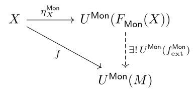 commutes.
We call \(\eta^{\mathsf{Mon}}_{X}\) the unit map (it depends on both the set \(X\) and the functor \(U^{\mathsf{Mon}}_{}\)) and \(f^{\mathsf{Mon}}_{\mathrm{ext}}\) the extension of \(f\).
Discussion 1.4.7. Start with a set \(X\). How can we equip it with a product when we have nothing else to work with? Say \(X = \{a, b, c\}\). What could be a sensible way to multiply these given no other structure? The reader is invited to try before reading on.
Say we want \(a \otimes b\). Could we just take \(a \otimes b \coloneqq ab\)? That is, can we just take concatenation (putting the letters next to each other) as a product? Let’s see if this holds up. \(a \otimes a = aa\), \((a \otimes b) \otimes c = (ab) \otimes c = abc = a \otimes (bc) = a \otimes (b \otimes c)\). This seems promising. It is associative (and non-commutative). What’s the identity? No letter of \(X\) will do: \(x \otimes a = xa\) is two letters long, never \(a\). The identity has to be the string with no letters at all, which is not an element of \(X\), but is something we have to add. Write \(\varepsilon\) for this empty string, the empty word. Then \(\varepsilon \otimes a = \varepsilon a = a = a \varepsilon = a \otimes \varepsilon\).
Notice that we have already left \(X\): \(aa\), \(abc\) and \(\varepsilon\) are not elements of \(X\). The monoid we are after lives on a larger set built from \(X\).
Discussion 1.4.8. We have the core idea to define this rigorously. Now we need to refine it. What’s the set for this monoid candidate? From \(X\) we grow to a set of all finite strings of elements in \(X\) (including the empty word, \(\varepsilon\)). Take a minute to make sure this is clear. We have \(\{\varepsilon, a, b, c, aa, bb, cc, ab, ac, \ldots\}\).
It will help us to cast this in terms of functions. Let \[[n] \coloneqq \{1, 2, \ldots, n\}, \qquad [0] = \varnothing\] then we see that each string of elements is a function \([n] \xrightarrow{w} X\). We call each such function a word (or a word on \(X\)).
Each word has a definite length, the \(n\) in its domain \([n]\); we will give it a name shortly, since it will be used repeatedly. We can now define our candidate free monoid.
Definition 1.4.9. For a set \(X\), the set of words on \(X\) is the set of all functions \([n] \to X\), for all \(n \in \mathbb{N}\): \[W(X) \coloneqq \bigcup_{n \in \mathbb{N}} \mathsf{Set}([n], X).\] The union is disjoint, since a function determines its domain. A word \(w\colon [n] \to X\) is the same thing as the \(n\)-tuple \((w(1), \ldots, w(n))\) of its letters, and we will often write it that way; the one function \([0] \to X\) is the empty word \(\varepsilon\).
Proposition 1.4.10. \(W(X)\) is a monoid under concatenation: for \(v\colon [n] \to X\) and \(w\colon [m] \to X\), \[v \frown w\colon [n + m] \to X, \qquad (v \frown w)(k) \coloneqq \begin{cases} v(k) & 1 \leq k \leq n, \\ w(k - n) & n < k \leq n + m, \end{cases}\] with unit the empty word \(\varepsilon\). In tuple notation, \((x_1, \ldots, x_n) \frown (y_1, \ldots, y_m) = (x_1, \ldots, x_n, y_1, \ldots, y_m)\).
Proof 1.4.11 (of Proposition 1.4.10). We have to show this multiplication is associative and the unit two sided. Exercise 1.4.3.
Definition 1.4.12. The length of a word \(w\colon [n] \to X\) is \(\ell(w) \coloneqq n\). This defines a function \(\ell\colon W(X) \to \mathbb{N}\). \(\ell(w) = 0\) exactly when \(w = \varepsilon\).
Lemma 1.4.13. \(\ell\colon W(X) \to (\mathbb{N}, +, 0)\) is a monoid homomorphism: \(\ell(v \frown w) = \ell(v) + \ell(w)\) and \(\ell(\varepsilon) = 0\).
Proof 1.4.14 (of Lemma 1.4.13). Both are read off the definitions: \(v \frown w\) has domain \([n + m]\) when \(v\) and \(w\) have domains \([n]\) and \([m]\), and \(\varepsilon\) has domain \([0]\).
Discussion 1.4.15. Now that we have a candidate monoid, we need our function \[X \xrightarrow{\delta^{\mathsf{Mon}}_{X}} U^{\mathsf{Mon}}_{}(W(X)).\] There is only one reasonable choice: send each element of \(X\) to the word of length one whose single letter it is, \[\begin{array}{rcl} X & \xrightarrow{\delta^{\mathsf{Mon}}_{X}} & U^{\mathsf{Mon}}_{}(W(X)) \\ x & \mapsto & (x), \end{array}\] where \((x)\) is the function \([1] \to X\) with \(1 \mapsto x\), that is, the one-tuple. We call the words \((x)\) the letters; they are the generators of \(W(X)\) in the sense of Principle 1.3.13. Our candidate solution is \((W(X), \delta^{\mathsf{Mon}}_X)\).
In tuple notation the product of letters is \((x_1) \frown (x_2) \frown \cdots \frown (x_n) = (x_1, x_2, \ldots, x_n)\), and we will usually drop the \(\frown\) between letters and write \((x_1)(x_2) \cdots (x_n)\). Note that \(\varepsilon\) is not a letter: it is the empty product of letters, the word with \(n = 0\).
Lemma 1.4.16. \(\{(x) \mid x \in X\}\) generates \(W(X)\), and each \(w \in W(X)\) has \(w = (x_1) \cdots (x_n)\) for some finite \(n\), uniquely so: \(n = \ell(w)\) and \(x_i = w(i)\).
Proof 1.4.17 (of Lemma 1.4.16). Let \(w \in W(X)\) and \(n = \ell(w)\). If \(n = 0\) then \(w = \varepsilon\), the empty product of letters. Otherwise set \(x_i \coloneqq w(i)\) for \(1 \leq i \leq n\). By Proposition 1.4.10 the product \((x_1)(x_2) \cdots (x_n)\) is the \(n\)-tuple \((x_1, \ldots, x_n)\), that is, the function \([n] \to X\) sending \(i\) to \(x_i = w(i)\); so it is \(w\). Hence every word is a product of letters, and the letters generate \(W(X)\).
The expression is forced: if \(w = (x_1) \cdots (x_n)\) then comparing domains gives \(n = \ell(w)\), and comparing values gives \(x_i = w(i)\).
We can now prove the following.
Theorem 1.4.18. \((W(X), X \xrightarrow{\delta^{\mathsf{Mon}}_{X}} U^{\mathsf{Mon}}_{}(W(X)))\) is initial in \(X \downarrow U^{\mathsf{Mon}}_{}\); that is, it is a free monoid on \(X\).
Strategy 1.4.19 (of Theorem 1.4.18). Consider an arbitrary \((M, X \xrightarrow{f} U^{\mathsf{Mon}}_{}(M))\) in \(X \downarrow U^{\mathsf{Mon}}_{}\). Principle 1.3.13 tells us where to look: the commutative diagram of Definition 1.4.6 forces, for \(x \in X\), \(f(x) = U^{\mathsf{Mon}}_{}(f^{\mathrm{cand}}_{\mathrm{ext}})((x))\) where, remember, \((x)\) is the one-letter word \([1] \to X\) mapping \(1\) to \(x\). We have just shown in Lemma 1.4.16 that each \(w \in W(X)\) is \((x_1)(x_2) \cdots (x_n)\) uniquely. Since \(f^{\mathrm{cand}}_{\mathrm{ext}}\) is to be a monoid homomorphism, \(f^{\mathrm{cand}}_{\mathrm{ext}}(w) = f(x_1) \otimes \cdots \otimes f(x_n)\), and \(f^{\mathrm{cand}}_{\mathrm{ext}}(\varepsilon) = 1_M\). That is our candidate. The proof checks that it is a monoid homomorphism, that it makes the diagram commute, and that it is the only one that does.
Proof 1.4.20 (of Theorem 1.4.18). Let \((M, X \xrightarrow{f} U^{\mathsf{Mon}}_{}(M))\) be an object of \(X \downarrow U^{\mathsf{Mon}}_{}\). Every word is \(w = (x_1)(x_2) \cdots (x_n)\) for a unique \(n\) and unique letters \(x_1, \ldots, x_n\) (Lemma 1.4.16), so \[\begin{array}{rcl} W(X) & \xrightarrow{f^{\mathrm{cand}}_{\mathrm{ext}}} & M \\ (x_1) \cdots (x_n) & \mapsto & f(x_1) \otimes \cdots \otimes f(x_n) \\ \varepsilon & \mapsto & 1_M \end{array}\] is well defined. It is a monoid homomorphism: it sends \(\varepsilon\) to \(1_M\), and if \(v = (x_1) \cdots (x_n)\) and \(w = (y_1) \cdots (y_m)\) then \[\begin{align*} f^{\mathrm{cand}}_{\mathrm{ext}}(v \frown w) &= f^{\mathrm{cand}}_{\mathrm{ext}}((x_1) \cdots (x_n)(y_1) \cdots (y_m)) \\ &= f(x_1) \otimes \cdots \otimes f(x_n) \otimes f(y_1) \otimes \cdots \otimes f(y_m) \\ &= f^{\mathrm{cand}}_{\mathrm{ext}}(v) \otimes f^{\mathrm{cand}}_{\mathrm{ext}}(w). \end{align*}\] It makes the diagram commute: for \(x \in X\), \(U^{\mathsf{Mon}}_{}(f^{\mathrm{cand}}_{\mathrm{ext}})(\delta^{\mathsf{Mon}}_{X}(x)) = f^{\mathrm{cand}}_{\mathrm{ext}}((x)) = f(x)\).
Finally, is \(f^{\mathrm{cand}}_{\mathrm{ext}}\) unique? Say \(f^{\mathrm{cand}}_1\) and \(f^{\mathrm{cand}}_2\) both make the diagram commute. Then \(f^{\mathrm{cand}}_1((x)) = f(x) = f^{\mathrm{cand}}_2((x))\) for all \(x \in X\). But \(f^{\mathrm{cand}}_1\) and \(f^{\mathrm{cand}}_2\) being monoid homomorphisms means for any \(w = (x_1) \cdots (x_n)\) \[\begin{align*} f^{\mathrm{cand}}_1(w) &= f^{\mathrm{cand}}_1((x_1) \cdots (x_n)) \\ &= f^{\mathrm{cand}}_1((x_1)) \otimes \cdots \otimes f^{\mathrm{cand}}_1((x_n)) \\ &= f(x_1) \otimes \cdots \otimes f(x_n) \\ &= f^{\mathrm{cand}}_2((x_1)) \otimes \cdots \otimes f^{\mathrm{cand}}_2((x_n)) \\ &= f^{\mathrm{cand}}_2((x_1) \cdots (x_n)) \\ &= f^{\mathrm{cand}}_2(w), \end{align*}\] and \(f^{\mathrm{cand}}_1(\varepsilon) = 1_M = f^{\mathrm{cand}}_2(\varepsilon)\); hence \(f^{\mathrm{cand}}_1 = f^{\mathrm{cand}}_2\), meaning \(f^{\mathrm{cand}}_{\mathrm{ext}}\) is the unique monoid homomorphism making the diagram commute. Hence \((W(X), X \xrightarrow{\delta^{\mathsf{Mon}}_{X}} U^{\mathsf{Mon}}_{}(W(X)))\) is initial in \(X \downarrow U^{\mathsf{Mon}}_{}\), that is, a free monoid on \(X\), and from now on we write \(f^{\mathsf{Mon}}_{\mathrm{ext}}\) for \(f^{\mathrm{cand}}_{\mathrm{ext}}\).
Example 1.4.21. Let \(X = \{x\}\). A word \(w\colon [n] \to \{x\}\) is determined by its length \(n\), since every letter is \(x\); write it \(x^n = (x)(x) \cdots (x)\) (\(n\) letters). Concatenation adds lengths, \(x^m x^n = x^{m+n}\), so \(\ell\) is a bijective homomorphism (Lemma 1.4.13), an isomorphism of monoids \(W(\{x\}) \cong (\mathbb{N}, +, 0)\). Given any monoid \(M\) and \(m \in M\), the unique extension of \(x \mapsto m\) sends \(x^n\) to \(m^n = m \otimes \cdots \otimes m\): a homomorphism out of the free monoid on one generator is just a choice of element, and its values are that element’s powers.
Example 1.4.22. Let \(X = \{a, b\}\). The words are \(\varepsilon, a, b, aa, ab, ba, bb, aaa, \ldots\), and \(ab \neq ba\), so \(W(X)\) is not commutative. A monoid homomorphism from \(W(X)\) to the \(2 \times 2\) real matrices under multiplication is determined by choosing two matrices \(A\) and \(B\) (the images of \(a\) and \(b\)); for instance the word \(abba\) goes to \(ABBA\). Nothing forces \(AB = BA\), which is exactly why the free monoid must not be commutative.
Exercises
Exercise 1.4.1. Show that the composite of two monoid homomorphisms is a monoid homomorphism, and that the identity function of a monoid is one. Conclude that \(\mathsf{Mon}\) is a category.
Exercise 1.4.2. Let \(\mathsf{C}\) be a category with exactly one object \(\ast\).
Show that \((\mathsf{C}(\ast, \ast), \circ, 1_\ast)\) is a monoid. Conversely, show that every monoid \((M, \otimes, 1_\otimes)\) arises this way from a category with one object whose arrows are the elements of \(M\).
Show that the monoid in (a) is a group exactly when every arrow of \(\mathsf{C}\) is an isomorphism.
Show that a monoid homomorphism \(M \to M'\) is the same thing as a functor between the corresponding one-object categories.
Exercise 1.4.3. Show that concatenation on \(W(X)\) is associative and that \(\varepsilon\) is a two-sided unit.
Exercise 1.4.4. Show that \(W(\varnothing)\) is the trivial monoid and that \(W(\{x\}) \cong (\mathbb{N}, +, 0)\).
Exercise 1.4.5. Show that \(W(X)\) is commutative if and only if \(X\) has at most one element.
Exercise 1.4.6. Let \(c\colon X \to U^{\mathsf{Mon}}_{}(\mathbb{N})\) be the constant function \(1\), where \(\mathbb{N}\) is a monoid under addition. Show that \(c^{\mathsf{Mon}}_{\mathrm{ext}} = \ell\), the length map of Definition 1.4.12.
1.5 The Monoid Algebra & the Composite
Discussion 1.5.1. We are now ready for the second part of the free algebra on a set problem. The first part mapped the set \(X\) to the monoid \(W(X)\) in a universal way. Now we need to map the monoid \(W(X)\) to an algebra in a universal way, and then check that the composite of the two universal maps is itself universal. The first step is the same sort of problem as before, with one twist. Our first two problems went \(\mathsf{Set}\to \mathsf{Vect}_K\) and \(\mathsf{Set}\to \mathsf{Mon}\), starting from no structure at all. This one goes \(\mathsf{Mon}\to \mathsf{Alg}_K\), and the structure we start with has to be respected.
The forgetful functor is now \(U^{\mathsf{Alg}}_{\mathsf{Mon}}\colon \mathsf{Alg}_K \to \mathsf{Mon}\), which takes an algebra and forgets its vector space structure, remembering its monoid structure (Definition 1.4.2), and sends an algebra homomorphism to itself, regarded as a monoid homomorphism. We state the problem for an arbitrary monoid \(M\), since nothing in it depends on \(M\) being \(W(X)\).
Definition 1.5.2. Let \(M\) be a monoid. A free algebra on the monoid \(M\) is an initial object \[(F^{\mathsf{Mon}}_{\mathsf{Alg}}(M), M \xrightarrow{\eta^{\mathsf{Alg},\mathsf{Mon}}_{M}} U^{\mathsf{Alg}}_{\mathsf{Mon}}(F^{\mathsf{Mon}}_{\mathsf{Alg}}(M)))\] of \(M \downarrow U^{\mathsf{Alg}}_{\mathsf{Mon}}\) (\(M\) also naming the functor \(\mathsf{1}\to \mathsf{Mon}\) that picks it out, as \(X\) did for sets).
That is, for every algebra \(A\) and monoid homomorphism \(f\colon M \to U^{\mathsf{Alg}}_{\mathsf{Mon}}(A)\) there is exactly one algebra homomorphism \[F^{\mathsf{Mon}}_{\mathsf{Alg}}(M) \xrightarrow{f^{\mathsf{Alg},\mathsf{Mon}}_{\mathrm{ext}}} A\] such that 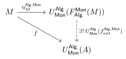 commutes.
We call \(\eta^{\mathsf{Alg},\mathsf{Mon}}_{M}\) the unit map and \(f^{\mathsf{Alg},\mathsf{Mon}}_{\mathrm{ext}}\) the extension of \(f\). The difference from Definitions 1.2.13 and 1.4.6 is that \(f\) is no longer an arbitrary function: it is a monoid homomorphism, and so is the unit map.
Discussion 1.5.3. We need a candidate: an algebra, together with a monoid homomorphism from \(M\) into its underlying monoid. For the vector space part we already know what to do. Take \(K^{(M)}\), the free vector space on the set \(M\), with its basis \(\{\delta_m \mid m \in M\}\) and the map \(m \mapsto \delta_m\) (§1.3 with \(M\) in place of \(X\)). What is new is that this map must now be a monoid homomorphism, \[\begin{array}{rcl} M & \xrightarrow{\delta^{\mathsf{Alg},\mathsf{Mon}}_{M}} & U^{\mathsf{Alg}}_{\mathsf{Mon}}(K^{(M)}) \\ m & \mapsto & \delta_m, \end{array}\] and \(K^{(M)}\) does not yet have a product for it to preserve.
Principle 1.3.13 says where to look: at the generators. For \(\delta^{\mathsf{Alg},\mathsf{Mon}}_{M}\) to be a monoid homomorphism we need, for all \(m, m' \in M\), \[\delta_m \ast \delta_{m'} = \delta_{m \otimes m'} \qquad\text{and}\qquad 1 = \delta_{1_M},\] whatever the product \(\ast\) on \(K^{(M)}\) turns out to be. That pins the product down on the basis, and bilinearity does the rest. For \(\phi, \psi \in K^{(M)}\), written as finite sums over their supports (Lemma 1.3.8), a bilinear product must satisfy \[\begin{align*} \phi \ast \psi &= \Bigl(\sum_{m \in \mathop{\mathrm{supp}}\phi} \phi(m)\, \delta_m\Bigr) \ast \Bigl(\sum_{m' \in \mathop{\mathrm{supp}}\psi} \psi(m')\, \delta_{m'}\Bigr) \\ &= \sum_{m \in \mathop{\mathrm{supp}}\phi} \sum_{m' \in \mathop{\mathrm{supp}}\psi} \phi(m)\, \psi(m')\, \delta_{m} \ast \delta_{m'} \\ &= \sum_{m \in \mathop{\mathrm{supp}}\phi} \sum_{m' \in \mathop{\mathrm{supp}}\psi} \phi(m)\, \psi(m')\, \delta_{m \otimes m'}, \end{align*}\] where the bilinearity is used in both slots in second line to expand the sums. So the one relation \(\delta_m \ast \delta_{m'} = \delta_{m \otimes m'}\) generates the whole multiplication, just as in §1.3 the values on the \(\delta_x\) generated the whole extension. The right-hand side is a finite sum of basis vectors, so it lies in \(K^{(M)}\).
“Bilinearity does the rest” deserves to be made precise, and the precise version is useful well beyond this section: a function of two variables on sets extends uniquely to a bilinear function on the free vector spaces. We prove that first, then return to \(K^{(M)}\).
Theorem 1.5.4 (Bilinear Extension). Take sets \(X, Y, Z\) and a function \(X \times Y \xrightarrow{f} Z\). Then there exists a unique bilinear function \[K^{(X)} \times K^{(Y)} \xrightarrow{f^{\mathrm{bilin}}_{\mathrm{ext}}} K^{(Z)}\] satisfying \(f^{\mathrm{bilin}}_{\mathrm{ext}}(\delta_x, \delta_y) = \delta_{f(x, y)}\).
Strategy 1.5.5 (of Theorem 1.5.4). The two key facts we exploit are that \(f^{\mathrm{bilin}}_{\mathrm{ext}}\) is to be bilinear and that the supports are all finite. Say \((\phi, \psi) \in K^{(X)} \times K^{(Y)}\), with \(\phi = \sum_{x \in \mathop{\mathrm{supp}}\phi} \phi(x)\, \delta_x\) and \(\psi = \sum_{y \in \mathop{\mathrm{supp}}\psi} \psi(y)\, \delta_y\). Bilinearity, used twice, and the required values on the \(\delta\)’s force \[\begin{align*} f^{\mathrm{bilin}}_{\mathrm{ext}}(\phi, \psi) &= f^{\mathrm{bilin}}_{\mathrm{ext}}\Bigl(\sum_{x \in \mathop{\mathrm{supp}}\phi} \phi(x)\, \delta_x,\ \sum_{y \in \mathop{\mathrm{supp}}\psi} \psi(y)\, \delta_y\Bigr) \\ &= \sum_{x \in \mathop{\mathrm{supp}}\phi} \sum_{y \in \mathop{\mathrm{supp}}\psi} \phi(x)\, \psi(y)\, f^{\mathrm{bilin}}_{\mathrm{ext}}(\delta_x, \delta_y) \\ &= \sum_{x \in \mathop{\mathrm{supp}}\phi} \sum_{y \in \mathop{\mathrm{supp}}\psi} \phi(x)\, \psi(y)\, \delta_{f(x, y)}. \end{align*}\] So there is only one candidate, which is uniqueness. What remains is to check that this candidate really is bilinear; that is where finite support comes in.
Proof 1.5.6 (of Theorem 1.5.4). Define \[\begin{array}{rcl} K^{(X)} \times K^{(Y)} & \xrightarrow{f^{\mathrm{bilin}}_{\mathrm{ext}}} & K^{(Z)} \\ (\phi, \psi) & \mapsto & \displaystyle\sum_{x \in \mathop{\mathrm{supp}}\phi} \sum_{y \in \mathop{\mathrm{supp}}\psi} \phi(x)\, \psi(y)\, \delta_{f(x, y)}. \end{array}\] Because \(f(x,y)\in Z\) and the supports are finite, the value is a finite linear combination of the \(\delta_z\), \(z \in Z\), so it has finite support, that is, it is an element of \(K^{(Z)}\). For \(\phi = \delta_x\) and \(\psi = \delta_y\) the supports are \(\{x\}\) and \(\{y\}\) and the sum is the single term \(\delta_{f(x, y)}\).
Bilinearity means \(f^{\mathrm{bilin}}_{\mathrm{ext}}(\lambda\phi_1 + \phi_2, \psi) = \lambda f^{\mathrm{bilin}}_{\mathrm{ext}}(\phi_1, \psi) + f^{\mathrm{bilin}}_{\mathrm{ext}}(\phi_2, \psi)\) and \(f^{\mathrm{bilin}}_{\mathrm{ext}}(\phi, \lambda\psi_1 + \psi_2) = \lambda f^{\mathrm{bilin}}_{\mathrm{ext}}(\phi, \psi_1) + f^{\mathrm{bilin}}_{\mathrm{ext}}(\phi, \psi_2)\). The proofs are the same, so we just do the first. Since \(\mathop{\mathrm{supp}}(\lambda\phi_1 + \phi_2) \subseteq \mathop{\mathrm{supp}}(\phi_1) \cup \mathop{\mathrm{supp}}(\phi_2)\) (Exercise 1.5.1), and \((\lambda\phi_1 + \phi_2)(x) = 0\) at every \(x \notin \mathop{\mathrm{supp}}(\lambda\phi_1 + \phi_2)\), we may sum over the larger finite set \(S \coloneqq \mathop{\mathrm{supp}}(\phi_1) \cup \mathop{\mathrm{supp}}(\phi_2)\) without changing the value: \[\begin{align*} f^{\mathrm{bilin}}_{\mathrm{ext}}(\lambda\phi_1 + \phi_2, \psi) &= \sum_{x \in S} \sum_{y \in \mathop{\mathrm{supp}}\psi} (\lambda\phi_1 + \phi_2)(x)\, \psi(y)\, \delta_{f(x, y)} \\ &= \lambda \sum_{x \in S} \sum_{y \in \mathop{\mathrm{supp}}\psi} \phi_1(x)\, \psi(y)\, \delta_{f(x, y)} \\ &\qquad + \sum_{x \in S} \sum_{y \in \mathop{\mathrm{supp}}\psi} \phi_2(x)\, \psi(y)\, \delta_{f(x, y)} \\ &= \lambda \sum_{x \in \mathop{\mathrm{supp}}\phi_1} \sum_{y \in \mathop{\mathrm{supp}}\psi} \phi_1(x)\, \psi(y)\, \delta_{f(x, y)} \\ &\qquad + \sum_{x \in \mathop{\mathrm{supp}}\phi_2} \sum_{y \in \mathop{\mathrm{supp}}\psi} \phi_2(x)\, \psi(y)\, \delta_{f(x, y)} \\ &= \lambda f^{\mathrm{bilin}}_{\mathrm{ext}}(\phi_1, \psi) + f^{\mathrm{bilin}}_{\mathrm{ext}}(\phi_2, \psi). \end{align*}\] The second equality is the pointwise definition of \(\lambda\phi_1 + \phi_2\) (Notation 1.3.2) and the splitting of a finite sum. The third drops from the first sum the terms with \(x \in S \setminus \mathop{\mathrm{supp}}(\phi_1)\), and from the second those with \(x \in S \setminus \mathop{\mathrm{supp}}(\phi_2)\); these terms are zero because \(\phi_1\) vanishes off \(\mathop{\mathrm{supp}}(\phi_1)\) and \(\phi_2\) off \(\mathop{\mathrm{supp}}(\phi_2)\). So \(f^{\mathrm{bilin}}_{\mathrm{ext}}\) is bilinear.
Uniqueness: if \(h\) is bilinear with \(h(\delta_x, \delta_y) = \delta_{f(x, y)}\), then expanding \(\phi\) and \(\psi\) over their supports and using bilinearity twice, \[\begin{align*} h(\phi, \psi) &= \sum_{x \in \mathop{\mathrm{supp}}\phi} \sum_{y \in \mathop{\mathrm{supp}}\psi} \phi(x)\, \psi(y)\, h(\delta_x, \delta_y) \\ &= \sum_{x \in \mathop{\mathrm{supp}}\phi} \sum_{y \in \mathop{\mathrm{supp}}\psi} \phi(x)\, \psi(y)\, \delta_{f(x, y)} = f^{\mathrm{bilin}}_{\mathrm{ext}}(\phi, \psi). \end{align*}\]
Corollary 1.5.7 (Multilinear Extension). Take sets \(X_1, \ldots, X_n, Y\) for \(n \in \mathbb{N}\) (so \(n\) finite) and a function \(X_1 \times X_2 \times \cdots \times X_n \xrightarrow{f} Y\). Then, there exists a unique multilinear extension  satisfying \(f^{\mathrm{multilin}}_{\mathrm{ext}}(\delta_{x_1}, \delta_{x_2}, \ldots, \delta_{x_n})
= \delta_{f(x_1, x_2, \ldots, x_n)}\).
Sketch 1.5.8 (of Corollary 1.5.7). The proof of Theorem 1.5.4 with \(n\) sums in place of two: multilinearity applied \(n\) times forces \[f^{\mathrm{multilin}}_{\mathrm{ext}}(\phi_1, \ldots, \phi_n) = \sum_{x_1 \in \mathop{\mathrm{supp}}\phi_1} \cdots \sum_{x_n \in \mathop{\mathrm{supp}}\phi_n} \phi_1(x_1) \cdots \phi_n(x_n)\, \delta_{f(x_1, \ldots, x_n)},\] which gives uniqueness, and linearity in the \(i\)-th argument, the others held fixed, is checked exactly as above. The details are Exercise 1.5.2.
Proposition 1.5.9. Let \(M\) be a monoid. Define the convolution product on \(K^{(M)}\) by \[\phi \ast \psi \coloneqq \sum_{m \in \mathop{\mathrm{supp}}\phi} \sum_{m' \in \mathop{\mathrm{supp}}\psi} \phi(m)\, \psi(m')\, \delta_{m \otimes m'}.\] With \(\ast\) as multiplication and \(\delta_{1_M}\) as unit, \(K^{(M)}\) is a unital, associative \(K\)-algebra, the monoid algebra of \(M\), which we write \(K[M]\); and \[M \xrightarrow{\delta^{\mathsf{Alg},\mathsf{Mon}}_{M}} U^{\mathsf{Alg}}_{\mathsf{Mon}}(K[M])\] is a monoid homomorphism into it.
Proof 1.5.10 (of Proposition 1.5.9). \(K^{(M)}\) is a vector space by Lemma 1.3.6. The product \(\ast\) is exactly the bilinear extension \(\otimes^{\mathrm{bilin}}_{\mathrm{ext}}\) of the multiplication \(\otimes\colon M \times M \to M\) of Theorem 1.5.4, with \(X = Y = Z = M\); so \(\ast\) is bilinear, and \(\delta_m \ast \delta_{m'} = \delta_{m \otimes m'}\).
Associativity. The two maps \[(\phi, \psi, \chi) \mapsto (\phi \ast \psi) \ast \chi \qquad\text{and}\qquad (\phi, \psi, \chi) \mapsto \phi \ast (\psi \ast \chi)\] are trilinear \(K^{(M)} \times K^{(M)} \times K^{(M)} \to K^{(M)}\), since \(\ast\) is linear in each argument. On basis elements they give \(\delta_{(m \otimes m') \otimes m''}\) and \(\delta_{m \otimes (m' \otimes m'')}\), which are equal because \(\otimes\) is associative in \(M\). So both are multilinear extensions of the same function \(M \times M \times M \to M\), \((m, m', m'') \mapsto m \otimes m' \otimes m''\), and by the uniqueness in Corollary 1.5.7 they are equal.
Unit. For \(\phi \in K^{(M)}\), \[\delta_{1_M} \ast \phi = \sum_{m' \in \mathop{\mathrm{supp}}\phi} \phi(m')\, \delta_{1_M \otimes m'} = \sum_{m' \in \mathop{\mathrm{supp}}\phi} \phi(m')\, \delta_{m'} = \phi,\] and \(\phi \ast \delta_{1_M} = \phi\) the same way.
Finally, \(\delta^{\mathsf{Alg},\mathsf{Mon}}_{M}(m \otimes m') = \delta_{m \otimes m'} = \delta_m \ast \delta_{m'}\) and \(\delta^{\mathsf{Alg},\mathsf{Mon}}_{M}(1_M) = \delta_{1_M}\) is the unit of \(K[M]\): these are the two conditions for a monoid homomorphism.
Now we prove the second half we need for the free algebra on a set problem.
Proposition 1.5.11. Let \(M\) be a monoid. The object \[(K[M], M \xrightarrow{\delta^{\mathsf{Alg},\mathsf{Mon}}_{M}} U^{\mathsf{Alg}}_{\mathsf{Mon}}(K[M]))\] is initial in \(M \downarrow U^{\mathsf{Alg}}_{\mathsf{Mon}}\); that is, it is a free algebra on the monoid \(M\).
Strategy 1.5.12 (of Proposition 1.5.11). Consider \((A, M \xrightarrow{f} U^{\mathsf{Alg}}_{\mathsf{Mon}}(A))\), with \(f\) a monoid homomorphism. We need a unique algebra homomorphism \(K[M] \xrightarrow{f^{\mathrm{cand}}_{\mathrm{ext}}} A\) making 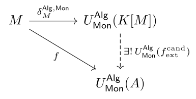 commute. We take the same strategy as before: use the diagram to derive a condition on the generators, use the condition to define \(f^{\mathrm{cand}}_{\mathrm{ext}}\) on all of \(K[M]\), and let the same condition give uniqueness. The diagram forces, for \(m \in M\), \[f(m) = U^{\mathsf{Alg}}_{\mathsf{Mon}}(f^{\mathrm{cand}}_{\mathrm{ext}})(\delta^{\mathsf{Alg},\mathsf{Mon}}_{M}(m))
= f^{\mathrm{cand}}_{\mathrm{ext}}(\delta_m),\] since \(U^{\mathsf{Alg}}_{\mathsf{Mon}}\) does not change where \(f^{\mathrm{cand}}_{\mathrm{ext}}\) sends elements. This is the key condition, \(f^{\mathrm{cand}}_{\mathrm{ext}}(\delta_m) = f(m)\), and since the \(\delta_m\) are a basis of \(K[M]\), linearity extends it to all of \(K[M]\) in exactly one way: it is the linear extension of §1.3. What is new is that this linear map must also be multiplicative, and that is what \(f\) being a monoid homomorphism buys.
Proof 1.5.13 (of Proposition 1.5.11). Let \((A, M \xrightarrow{f} U^{\mathsf{Alg}}_{\mathsf{Mon}}(A))\) be an object of \(M \downarrow U^{\mathsf{Alg}}_{\mathsf{Mon}}\). Regard \(f\) as a function into the vector space \(A\) and let \(f^{\mathrm{cand}}_{\mathrm{ext}}\) be its linear extension from Theorem 1.3.10, with \(M\) in place of \(X\): \[\begin{array}{rcl} K[M] & \xrightarrow{f^{\mathrm{cand}}_{\mathrm{ext}}} & A \\ \phi = \sum_{m \in \mathop{\mathrm{supp}}\phi} \phi(m)\, \delta_m & \mapsto & \sum_{m \in \mathop{\mathrm{supp}}\phi} \phi(m)\, f(m). \end{array}\] It is linear and \(f^{\mathrm{cand}}_{\mathrm{ext}}(\delta_m) = f(m)\). It is an algebra homomorphism: for \(\phi, \psi \in K[M]\), by the definition of \(\ast\), the fact that \(f\) is a monoid homomorphism, and bilinearity of \(\otimes\) in \(A\), \[\begin{align*} f^{\mathrm{cand}}_{\mathrm{ext}}(\phi \ast \psi) &= \sum_{m \in \mathop{\mathrm{supp}}\phi} \sum_{m' \in \mathop{\mathrm{supp}}\psi} \phi(m)\, \psi(m')\, f(m \otimes m') \\ &= \sum_{m \in \mathop{\mathrm{supp}}\phi} \sum_{m' \in \mathop{\mathrm{supp}}\psi} \phi(m)\, \psi(m')\, f(m) \otimes f(m') \\ &= \Bigl(\sum_{m \in \mathop{\mathrm{supp}}\phi} \phi(m)\, f(m)\Bigr) \otimes \Bigl(\sum_{m' \in \mathop{\mathrm{supp}}\psi} \psi(m')\, f(m')\Bigr) \\ &= f^{\mathrm{cand}}_{\mathrm{ext}}(\phi) \otimes f^{\mathrm{cand}}_{\mathrm{ext}}(\psi), \end{align*}\] and \(f^{\mathrm{cand}}_{\mathrm{ext}}(\delta_{1_M}) = f(1_M) = 1_A\). (The first line uses that \(f^{\mathrm{cand}}_{\mathrm{ext}}\) is linear and sends \(\delta_{m \otimes m'}\) to \(f(m \otimes m')\).) By construction \[f^{\mathrm{cand}}_{\mathrm{ext}}(\delta^{\mathsf{Alg},\mathsf{Mon}}_{M}(m)) = f^{\mathrm{cand}}_{\mathrm{ext}}(\delta_m) = f(m),\] so the diagram commutes.
Finally, is \(f^{\mathrm{cand}}_{\mathrm{ext}}\) unique? Say \(f^{\mathrm{cand}}_1\) and \(f^{\mathrm{cand}}_2\) both make the diagram commute. Then \(f^{\mathrm{cand}}_1(\delta_m) = f(m) = f^{\mathrm{cand}}_2(\delta_m)\) for all \(m \in M\), and for any \(\phi \in K[M]\) \[\begin{align*} f^{\mathrm{cand}}_1(\phi) &= f^{\mathrm{cand}}_1\Bigl(\sum_{m \in \mathop{\mathrm{supp}}\phi} \phi(m)\, \delta_m\Bigr) = \sum_{m \in \mathop{\mathrm{supp}}\phi} \phi(m)\, f^{\mathrm{cand}}_1(\delta_m) \\ &= \sum_{m \in \mathop{\mathrm{supp}}\phi} \phi(m)\, f(m) \\ &= \sum_{m \in \mathop{\mathrm{supp}}\phi} \phi(m)\, f^{\mathrm{cand}}_2(\delta_m) = f^{\mathrm{cand}}_2(\phi), \end{align*}\] where the crucial second equality is because \(f^{\mathrm{cand}}_1\) is an algebra homomorphism, hence linear. So \(f^{\mathrm{cand}}_1 = f^{\mathrm{cand}}_2\), meaning \(f^{\mathrm{cand}}_{\mathrm{ext}}\) is the unique algebra homomorphism making the diagram commute. Hence \((K[M], \delta^{\mathsf{Alg},\mathsf{Mon}}_{M})\) is a free algebra on the monoid \(M\), and from now on we write \(f^{\mathsf{Alg},\mathsf{Mon}}_{\mathrm{ext}}\) for \(f^{\mathrm{cand}}_{\mathrm{ext}}\).
Discussion 1.5.14. We are now almost done. We need to put our two constructions — the free monoid on a set and the free algebra on a monoid — together to solve the free algebra on a set problem: an initial object in \(X \downarrow U^{\mathsf{Alg}}_{}\), 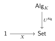 where \(U^{\mathsf{Alg}}_{}\) applied to an algebra remembers only its set. The candidate is \(K[W(X)]\), and the unit map is the composite of the two unit maps we have, \[\begin{array}{rcccl}
X & \xrightarrow{\delta^{\mathsf{Mon}}_{X}} & U^{\mathsf{Mon}}_{}(W(X))
& \xrightarrow{U^{\mathsf{Mon}}_{}(\delta^{\mathsf{Alg},\mathsf{Mon}}_{W(X)})} & U^{\mathsf{Alg}}_{}(K[W(X)]) \\
x & \mapsto & (x) & \mapsto & \delta_{(x)},
\end{array}\] which we call \(\delta^{\mathsf{Alg}}_{X}\). Here we have used that \(U^{\mathsf{Alg}}_{} = U^{\mathsf{Mon}}_{} \circ U^{\mathsf{Alg}}_{\mathsf{Mon}}\): an algebra homomorphism regarded as a monoid homomorphism and then as a function is the same function as the algebra homomorphism regarded as a function directly.
Rather than chase the two universal properties through diagrams specific to this case, we prove once that free objects compose. The lemma is stated for abstract categories; in our case \(\mathsf{A} = \mathsf{Set}\), \(\mathsf{B} = \mathsf{Mon}\), \(\mathsf{C} = \mathsf{Alg}_K\), \(U_1 = U^{\mathsf{Alg}}_{\mathsf{Mon}}\) and \(U_2 = U^{\mathsf{Mon}}_{}\).
Lemma 1.5.15 (Free objects compose). Let \(U_1\colon \mathsf{C} \to \mathsf{B}\) and \(U_2\colon \mathsf{B} \to \mathsf{A}\) be functors and \(U \coloneqq U_2 \circ U_1\colon \mathsf{C} \to \mathsf{A}\). Let \(a\) be an object of \(\mathsf{A}\). Suppose \[\begin{align*} (b, a \xrightarrow{\eta} U_2(b)) &\text{ is initial in } a \downarrow U_2, \text{ and} \\ (c, b \xrightarrow{\eta'} U_1(c)) &\text{ is initial in } b \downarrow U_1. \end{align*}\] Then \((c, a \xrightarrow{U_2(\eta') \circ \eta} U(c))\) is initial in \(a \downarrow U\).
Proof 1.5.16 (of Lemma 1.5.15). Let \((c', a \xrightarrow{f} U(c'))\) be an object of \(a \downarrow U\). We must show there is exactly one arrow \(g\colon c \to c'\) in \(\mathsf{C}\) with \(U(g) \circ U_2(\eta') \circ \eta = f\). The whole argument is the diagram 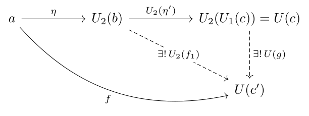 read twice, once for existence and once for uniqueness.
Existence. Since \(U(c') = U_2(U_1(c'))\), the pair \((U_1(c'), f)\) is an object of \(a \downarrow U_2\), so by the first universal property there is an arrow \(f_1\colon b \to U_1(c')\) in \(\mathsf{B}\) with \(U_2(f_1) \circ \eta = f\). Now \((c', f_1)\) is an object of \(b \downarrow U_1\), so by the second universal property there is an arrow \(g\colon c \to c'\) in \(\mathsf{C}\) with \(U_1(g) \circ \eta' = f_1\). Applying \(U_2\) to this last equation and composing with \(\eta\), \[U(g) \circ U_2(\eta') \circ \eta = U_2(U_1(g) \circ \eta') \circ \eta = U_2(f_1) \circ \eta = f.\]
Uniqueness. Suppose \(g'\colon c \to c'\) also satisfies \(U(g') \circ U_2(\eta') \circ \eta = f\). Then \(U_1(g') \circ \eta'\) is an arrow \(b \to U_1(c')\) in \(\mathsf{B}\), and \(U_2(U_1(g') \circ \eta') \circ \eta = f\), so it is an arrow \((b, \eta) \to (U_1(c'), f)\) in \(a \downarrow U_2\). By uniqueness in the first universal property, \(U_1(g') \circ \eta' = f_1\). So \(g'\) is an arrow \((c, \eta') \to (c', f_1)\) in \(b \downarrow U_1\), and by uniqueness in the second universal property, \(g' = g\).
Theorem 1.5.17. \((K[W(X)], X \xrightarrow{\delta^{\mathsf{Alg}}_{X}} U^{\mathsf{Alg}}_{}(K[W(X)]))\) is initial in \(X \downarrow U^{\mathsf{Alg}}_{}\); that is, it is a free algebra on \(X\). The extension of a function \(f\colon X \to U^{\mathsf{Alg}}_{}(A)\) is the extension of its extension: \[f^{\mathsf{Alg}}_{\mathrm{ext}} = (f^{\mathsf{Mon}}_{\mathrm{ext}})^{\mathsf{Alg},\mathsf{Mon}}_{\mathrm{ext}},\] where \(f^{\mathsf{Mon}}_{\mathrm{ext}}\colon W(X) \to U^{\mathsf{Alg}}_{\mathsf{Mon}}(A)\) is the monoid homomorphism extending \(f\) regarded as a function into the monoid \(A\).
Proof 1.5.18 (of Theorem 1.5.17). Apply Lemma 1.5.15 with \(\mathsf{A} = \mathsf{Set}\), \(\mathsf{B} = \mathsf{Mon}\), \(\mathsf{C} = \mathsf{Alg}_K\), \(U_1 = U^{\mathsf{Alg}}_{\mathsf{Mon}}\), \(U_2 = U^{\mathsf{Mon}}_{}\), so that \(U = U^{\mathsf{Alg}}_{}\); with \(a = X\) and \((b, \eta) = (W(X), \delta^{\mathsf{Mon}}_{X})\), initial by Theorem 1.4.18; and with \((c, \eta') = (K[W(X)], \delta^{\mathsf{Alg},\mathsf{Mon}}_{W(X)})\), initial by Proposition 1.5.11 with \(M = W(X)\). The composite unit \(U_2(\eta') \circ \eta\) is \(\delta^{\mathsf{Alg}}_{X}\), and the arrow \(g\) constructed in the lemma’s proof is \((f^{\mathsf{Mon}}_{\mathrm{ext}})^{\mathsf{Alg},\mathsf{Mon}}_{\mathrm{ext}}\).
Example 1.5.19. For \(X = \{x\}\), \(W(\{x\}) = \{x^n\}\) and \(\delta_{x^m} \ast \delta_{x^n} = \delta_{x^{m+n}}\). Matching \(\delta_{x^n}\) with the monomial \(x^n\) identifies \(K[W(\{x\})]\) with the polynomial algebra \(K[x]\), and convolution with polynomial multiplication. The free algebra on one generator is the polynomial algebra, and an algebra homomorphism \(K[x] \to A\) is the same as a choice of one element of \(A\) (“evaluate at \(a\)”).
Example 1.5.20. For \(X = \{x, y\}\), an element of \(K[W(X)]\) is a finite linear combination of words in \(x\) and \(y\), and \(\delta_x \ast \delta_y = \delta_{xy} \neq \delta_{yx} = \delta_y \ast \delta_x\). So \(K[W(X)]\) is the algebra of polynomials in non-commuting variables, usually written \(K\langle x, y \rangle\). An algebra homomorphism to the \(2 \times 2\) matrices is a choice of any two matrices, commuting or not. This algebra is the starting point for the tensor algebra in the next chapter.
Example 1.5.21. Not every monoid algebra is free. Let \(C_2 = \{1, s\}\) be the two-element monoid with \(s \otimes s = 1\) (and \(1\) the unit). Then \(K[C_2]\) is two-dimensional, with basis \(\delta_1, \delta_s\), unit \(\delta_1\), and \[\delta_s \ast \delta_s = \delta_{s \otimes s} = \delta_1.\] So \(K[C_2]\) is a commutative algebra with a generator whose square is the unit, and an algebra homomorphism \(K[C_2] \to A\) is a choice of an element \(a \in A\) with \(a \otimes a = 1_A\) (by Proposition 1.5.11, since a monoid homomorphism \(C_2 \to U^{\mathsf{Alg}}_{\mathsf{Mon}}(A)\) is exactly such a choice). Compare the free algebra on one generator, \(K[t]\), where the generator satisfies no relation at all. Algebras with generators squaring to a scalar are the subject of this book; this is the smallest one.
Exercises
Exercise 1.5.1. Show that \(\mathop{\mathrm{supp}}(\lambda\phi_1 + \phi_2) \subseteq \mathop{\mathrm{supp}}(\phi_1) \cup \mathop{\mathrm{supp}}(\phi_2)\), and give an example where the inclusion is strict.
Exercise 1.5.2. Prove Corollary 1.5.7.
Exercise 1.5.3. Show that \(K[M]\) is commutative if and only if the monoid \(M\) is commutative.
Exercise 1.5.4. Show that \(F^{}_{\mathsf{Alg}}(\varnothing) \cong K\).
Exercise 1.5.5. In \(K[W(\{a, b\})]\), compute \((\delta_a + \delta_b) \ast (\delta_a - \delta_b)\) and \((\delta_a - \delta_b) \ast (\delta_a + \delta_b)\), and compare.
Exercise 1.5.6.
Show that \(U^{\mathsf{Alg}}_{\mathsf{Mon}}\), which sends an algebra to its underlying monoid and an algebra homomorphism to itself, is a functor \(\mathsf{Alg}_K \to \mathsf{Mon}\), and that \(U^{\mathsf{Alg}}_{} = U^{\mathsf{Mon}}_{} \circ U^{\mathsf{Alg}}_{\mathsf{Mon}}\).
Let \(p\colon M \to M'\) be a monoid homomorphism. Using only the universal property of \(K[M]\), show that there is a unique algebra homomorphism \(K[M] \to K[M']\) sending \(\delta_m\) to \(\delta_{p(m)}\), and that this assignment respects composition and identities.
Exercise 1.5.7. The convolution formula was written for finitely supported \(\phi, \psi\). Try it on all of \(K^M\): for \(\phi, \psi \in K^M\) set \[(\phi \ast \psi)(m) \coloneqq \sum_{m_1 \otimes m_2 = m} \phi(m_1)\, \psi(m_2),\] the sum over all pairs \((m_1, m_2)\) with \(m_1 \otimes m_2 = m\).
Check that on \(K^{(M)}\) this agrees with the convolution product of Proposition 1.5.9.
For \(M = (\mathbb{N}, +, 0)\), show the sum is finite for every \(\phi, \psi \in K^{\mathbb{N}}\), so that \(K^{\mathbb{N}}\) becomes an algebra containing \(K[\mathbb{N}] \cong K[t]\). (It is the algebra of formal power series, written \(K[[t]]\).)
For \(M = (\mathbb{Z}, +, 0)\), show the sum can be infinite, so the formula does not define a product on \(K^{\mathbb{Z}}\).
So finite support is what makes convolution well defined on an arbitrary monoid.
Exercise 1.5.8. Remark 1.4.4 warned that making \(X\) a vector space first and then taking the free monoid on the underlying set of \(K^{(X)}\) is not a route to the free algebra. Let \(X = \{x\}\) and let \(B \coloneqq K[W(U^{\mathsf{Vect}}_{}(K^{(X)}))]\), the monoid algebra of the free monoid on the set of all vectors of \(K^{(X)} \cong K\).
Show that \(B\) has a letter \((\lambda)\) for every scalar \(\lambda \in K\), and that the \(\delta_{(\lambda)}\) are linearly independent in \(B\). Conclude that \(B\) is not isomorphic to \(K[t] = F^{}_{\mathsf{Alg}}(X)\) when \(K\) is infinite (compare the dimensions of the degree-one parts), and that in \(B\) the letter \((\lambda)\) bears no relation to \(\lambda\, \delta_{(1)}\).
Where does the route break? Identify the step at which the vector space structure of \(K^{(X)}\) was forgotten rather than respected.
1.6 Graded Algebras
Discussion 1.6.1. The algebra \(K[W(X)]\) we have built carries additional structure that it will be beneficial for us to highlight. Recall that \(\{\delta_w \mid w \in W(X)\}\) forms a basis for \(K[W(X)]\), and that each word has a length \(\ell(w)\) (Definition 1.4.12). Consider the monoid structure of the natural numbers under addition (so the product in this case is normal addition of natural numbers). With that structure \(\ell\colon W(X) \to \mathbb{N}\) is a monoid homomorphism (Lemma 1.4.13): the length of a concatenation is the sum of the lengths. In fact \(\ell\) is the canonical extension of the constant function \(1\) on \(X\): for \(c\colon X \to U^{\mathsf{Mon}}_{}(\mathbb{N})\), \(x \mapsto 1\), we have \(\ell = c^{\mathsf{Mon}}_{\mathrm{ext}}\) (Exercise 1.4.6).
Length sorts the basis. Each \(\delta_w\) sits at level \(\ell(w)\), so \(K[W(X)]\) splits into pieces, one for each \(n \in \mathbb{N}\), spanned by the \(\delta_w\) with \(\ell(w) = n\), and every element is a finite sum of pieces of different levels. That is the first structure: a vector space cut into levels indexed by the natural numbers. We call such a structure on a vector space a grading, and \(K[W(X)]\) is then a graded vector space. But \(K[W(X)]\) has a product too. The second structure consists of the fact that the product respects the grading, which makes \(K[W(X)]\) a graded algebra. On basis elements \(\delta_v \ast \delta_w = \delta_{v \frown w}\), and \(\ell(v \frown w) = \ell(v) + \ell(w)\), so multiplying a level-\(n\) element by a level-\(m\) element lands in level \(n + m\), and the unit \(\delta_\varepsilon\) sits at level \(0\). We formally define both structures first, in general, and then prove that \(K[W(X)]\) has them. These are \(\mathbb{N}\)-graded (other gradings will later be defined), but in general graded without qualification means \(\mathbb{N}\)-graded.
Definition 1.6.2. A vector space \(V\) is a graded vector space if \[V = \bigoplus_{n=0}^{\infty} V_n\] for subspaces \(V_n\). Each \(v \in V\) is then in exactly one way a finite sum \[v = \sum_{n=0}^{\infty} v_n, \qquad v_n \in V_n,\] with only finitely many \(v_n\) nonzero. We write \(\langle v \rangle_n \coloneqq v_n\) for the degree-\(n\) part of \(v\), and \(\langle V \rangle_n \coloneqq V_n\) for the degree-\(n\) part of \(V\). Elements of \(V_n\) are called homogeneous of degree \(n\).
Definition 1.6.3. The category \(\mathsf{GrVect}_K\) consists of graded vector spaces as objects with arrows \[V = \bigoplus_{n=0}^{\infty} V_n \xrightarrow{f} W = \bigoplus_{n=0}^{\infty} W_n\] linear maps such that \(f(V_n) \subseteq W_n\) for all \(n \in \mathbb{N}\).
Exercise 1.6.2 asks the reader to confirm this is a category, and Exercise 1.6.1 to define graded vector spaces in a more categorical manner. It will be useful to note an equivalent way to characterize graded vector spaces.
Definition 1.6.4. A projection operator or an idempotent on a vector space \(V\) is a linear map \(V \xrightarrow{p} V\) such that \[p^2 = p, \qquad\text{where } p^2 \coloneqq p \circ p.\] A complete system of orthogonal idempotents, or a decomposition of the identity, is a family of idempotents \(\{p_n\}_{n=0}^{\infty}\) such that \[p_m \circ p_n = 0 \quad (m \neq n) \qquad\text{and}\qquad \sum_{n=0}^{\infty} p_n = 1_V \text{ pointwise}.\] The first condition is orthogonality; it is purely algebraic, and no inner product or quadratic form is involved. The second means that for any particular \(v \in V\) only finitely many \(p_n(v)\) are non-zero, and they sum to \(v\).
Discussion 1.6.5. A grading \(V = \bigoplus_n V_n\) gives the complete system \(\{\langle - \rangle_n\}_{n=0}^{\infty}\) of its degree projections, and conversely a complete system of orthogonal idempotents gives a grading with \(V_n \coloneqq p_n(V)\); we leave it as an exercise (Exercise 1.6.3) that these two constructions are inverse to each other, so that our definition of a graded vector space is equivalent to having a complete system of idempotents.
A graded vector space is composed of separate pieces of different degrees. When the space is an algebra, we also want the product to respect the pieces. We can extend the idea of a graded vector space to include algebras too.
Definition 1.6.6. A graded algebra is a (unital, associative) \(K\)-algebra \(A\) whose underlying vector space is graded, \(A = \bigoplus_{n=0}^{\infty} A_n\), such that \[A_n A_m \subseteq A_{n+m},\] meaning \(a \otimes b \in A_{n+m}\) whenever \(a \in A_n\) and \(b \in A_m\), and the multiplicative identity \(1_A \in A_0\).
Exercise 1.6.4 asks the reader to show \(1_A \in A_0\) is automatic from the other structure in the definition. We can again package graded algebras into a category.
Definition 1.6.7. The category \(\mathsf{GrAlg}_K\) consists of graded \(K\)-algebras with arrows \[A = \bigoplus_{n=0}^{\infty} A_n \xrightarrow{f} B = \bigoplus_{n=0}^{\infty} B_n\] algebra homomorphisms such that \(f(A_n) \subseteq B_n\) for all \(n \in \mathbb{N}\).
Discussion 1.6.8. We now return to \(K[W(X)]\) and make the levels of Discussion 1.6.1 precise. Let \[W_n(X) \coloneqq \{\, w \in W(X) \mid \ell(w) = n \,\}\] be the words of length \(n\), and \[\langle K[W(X)] \rangle_n \coloneqq \{\, \phi \in K[W(X)] \mid \mathop{\mathrm{supp}}(\phi) \subseteq W_n(X) \,\}\] the functions supported on words of length \(n\). In particular, \(\langle K[W(X)] \rangle_0 = K\,\delta_\varepsilon\), spanned by the empty word, and \(W_1(X)\) is the set of letters \((x)\). For \(\phi \in K[W(X)]\) let \(\langle \phi \rangle_n\) be the function that agrees with \(\phi\) on \(W_n(X)\) and is \(0\) elsewhere; it lies in \(\langle K[W(X)] \rangle_n\), and \(\phi \mapsto \langle \phi \rangle_n\) is linear. The notation anticipates the following propositions, which say these are the degree-\(n\) projections of a grading that the product respects.
Proposition 1.6.9. The maps \(\langle - \rangle_n\colon K[W(X)] \to K[W(X)]\), \(n \in \mathbb{N}\), form a complete system of orthogonal idempotents:
each \(\langle - \rangle_n\) is linear;
\(\langle - \rangle_n \circ \langle - \rangle_n = \langle - \rangle_n\);
\(\langle - \rangle_m \circ \langle - \rangle_n = 0\) for \(m \neq n\);
\(\sum_{n=0}^{\infty} \langle - \rangle_n = 1_{K[W(X)]}\) pointwise (in the sense of Definition 1.6.4).
Proof 1.6.10 (a). Linearity is pointwise: \(\langle \lambda\phi + \psi \rangle_n\) and \(\lambda \langle \phi \rangle_n + \langle \psi \rangle_n\) agree on \(W_n(X)\) and are \(0\) off it.
(b) Restricting to \(W_n(X)\) twice is the same as restricting once, so \(\langle \langle \phi \rangle_n \rangle_n = \langle \phi \rangle_n\).
(c) For \(m \neq n\), \(\langle \phi \rangle_n\) is \(0\) off \(W_n(X)\), and \(W_m(X) \cap W_n(X) = \varnothing\), so \(\langle \langle \phi \rangle_n \rangle_m = 0\).
(d) Pointwise means two things for a given \(\phi \in K[W(X)]\): only finitely many \(\langle \phi \rangle_n\) are nonzero, and they sum to \(\phi\). The first is where we use that elements of \(K[W(X)]\) have finite support: \(\langle \phi \rangle_n \neq 0\) only if some word of length \(n\) lies in \(\mathop{\mathrm{supp}}(\phi)\), and a finite set of words has finitely many lengths. (On all of \(K^{W(X)}\) the same maps are still orthogonal idempotents, but a function supported on words of every length has infinitely many nonzero pieces, and the sum does not make sense.) For the second, both \(\sum_n \langle \phi \rangle_n\) and \(\phi\) are functions on \(W(X)\), and at a word of length \(n\) only the \(n\)th term of the sum is nonzero, where it equals \(\phi\).
Discussion 1.6.11. By Exercise 1.6.3, \(K[W(X)]\) is therefore a graded vector space, \[K[W(X)] = \bigoplus_{n=0}^{\infty} \langle K[W(X)] \rangle_n,\] with degree-\(n\) part the image of \(\langle - \rangle_n\), which is exactly \(\langle K[W(X)] \rangle_n\), the functions supported on words of length \(n\). In this grading, \(\langle \phi \rangle_n\) in the sense of Definition 1.6.2 is the \(\langle \phi \rangle_n\) we defined, so the notation is consistent.
It is worth noticing what did the work. Parts (a)–(c) of Proposition 1.6.9 are about the sets \(W_n(X)\): they partition \(W(X)\), and restriction to the parts of a partition is always a family of orthogonal idempotents. Part (d) is about the elements of \(K[W(X)]\): finite support is what makes every \(\phi\) a finite sum of its pieces, which is what a direct sum requires. This is the same finiteness that made the convolution product well defined in §1.5. It remains to see that the product respects the grading.
Proposition 1.6.12. With this grading, \(K[W(X)]\) is a graded algebra:
if \(\phi \in \langle K[W(X)] \rangle_n\) and \(\psi \in \langle K[W(X)] \rangle_m\), then \(\phi \ast \psi \in \langle K[W(X)] \rangle_{n+m}\);
the unit \(\delta_\varepsilon\) lies in \(\langle K[W(X)] \rangle_0\).
Proof 1.6.13 (a). On basis elements, \(\delta_v \ast \delta_w = \delta_{v \frown w}\) (Proposition 1.5.9 with \(M = W(X)\)) and \(\ell(v \frown w) = \ell(v) + \ell(w)\) (Lemma 1.4.13), so for \(v \in W_n(X)\) and \(w \in W_m(X)\) the product \(\delta_v \ast \delta_w\) lies in \(\langle K[W(X)] \rangle_{n+m}\). In general \(\phi = \sum_{v \in \mathop{\mathrm{supp}}\phi} \phi(v)\, \delta_v\) with \(\mathop{\mathrm{supp}}\phi \subseteq W_n(X)\) and \(\psi = \sum_{w \in \mathop{\mathrm{supp}}\psi} \psi(w)\, \delta_w\) with \(\mathop{\mathrm{supp}}\psi \subseteq W_m(X)\), so by bilinearity \[\phi \ast \psi = \sum_{v \in \mathop{\mathrm{supp}}\phi} \sum_{w \in \mathop{\mathrm{supp}}\psi} \phi(v)\, \psi(w)\, \delta_{v \frown w}\] is a linear combination of elements of the subspace \(\langle K[W(X)] \rangle_{n+m}\).
(b) \(\ell(\varepsilon) = 0\).
Discussion 1.6.14. Having cut \(K[W(X)]\) into pieces, we should look at the pieces. Degree \(0\) is \(K\,\delta_\varepsilon\), a copy of \(K\). Degree \(1\) is spanned by the \(\delta_{(x)}\) for the letters \((x)\), one for each \(x \in X\), so it is a copy of the free vector space \(K^{(X)}\) of §1.3; this is the piece in which \(X\) itself sits, and it is the one that will matter when we return to the universal property. The pattern continues: a word of length \(n\) is an \(n\)-tuple of letters, so degree \(n\) should be the free vector space on \(X^n\). The next proposition makes this precise and, as a consequence, counts dimensions. (Once we have tensor products, \(K^{(X^n)}\) will reappear as the \(n\)-fold tensor power of \(K^{(X)}\), and \(K[W(X)]\) as the tensor algebra.)
Proposition 1.6.15. \(\langle K[W(X)] \rangle_n \cong K^{(X^n)}\) as vector spaces, via \(\delta_w \mapsto \delta_{(w(1), \ldots, w(n))}\). If \(X\) has \(k\) elements, then \(\dim(\langle K[W(X)] \rangle_n) = k^n\).
Proof 1.6.16 (of Proposition 1.6.15). There are two steps. First, restriction to \(W_n(X)\) and extension by zero, \[\begin{array}{rcl} \langle K[W(X)] \rangle_n & \longrightarrow & K^{(W_n(X))} \\ \phi & \mapsto & \phi|_{W_n(X)}, \end{array} \qquad \begin{array}{rcl} K^{(W_n(X))} & \longrightarrow & \langle K[W(X)] \rangle_n \\ \psi & \mapsto & \psi_{\mathrm{all}}, \end{array}\] where \(\psi_{\mathrm{all}} = \psi\) on \(W_n(X)\) and \(\psi_{\mathrm{all}} = 0\) otherwise, are linear and inverse to each other (Exercise 1.6.6). This gives \(\langle K[W(X)] \rangle_n \cong K^{(W_n(X))}\), sending \(\delta_w\) as a function on \(W(X)\) to \(\delta_w\) as a function on \(W_n(X)\).
Second, \(W_n(X) = \mathsf{Set}([n], X)\) by Definition 1.4.9, and a function \([n] \to X\) is the same thing as the \(n\)-tuple of its values: \(w \mapsto (w(1), \ldots, w(n))\) is a bijection \(W_n(X) \to X^n\), with inverse \((x_1, \ldots, x_n) \mapsto (x_1) \frown \cdots \frown (x_n)\). A bijection of sets induces a linear isomorphism of the free vector spaces on them, \(K^{(W_n(X))} \cong K^{(X^n)}\) with \(\delta_w \mapsto \delta_{(w(1), \ldots, w(n))}\) (Exercise 1.6.5).
Putting these two together gives \(\langle K[W(X)] \rangle_n \cong K^{(W_n(X))} \cong K^{(X^n)}\). We leave the dimension argument as an exercise (Exercise 1.6.7).
Discussion 1.6.17. We only have one more result before we close this chapter. We have shown in the previous section that \((K[W(X)], X \xrightarrow{\delta^{\mathsf{Alg}}_{X}} U^{\mathsf{Alg}}_{}(K[W(X)]))\) is initial in \(X \downarrow U^{\mathsf{Alg}}_{}\). The interesting remaining result is that this is not the only comma category where \(K[W(X)]\) is initial.
Exercise 1.6.8 asks the reader to prove that \[\begin{array}{rcl} \mathsf{GrAlg}_K & \xrightarrow{\langle - \rangle_n} & \mathsf{Vect}_K \\ A = \bigoplus_{n=0}^{\infty} A_n & \mapsto & \langle A \rangle_n = A_n \end{array}\] is a functor for all \(n\). We are concerned with the composite functor \[\begin{array}{rcccl} \mathsf{GrAlg}_K & \xrightarrow{\langle - \rangle_1} & \mathsf{Vect}_K & \xrightarrow{U^{\mathsf{Vect}}_{}} & \mathsf{Set}\\ A & \mapsto & A_1 & \mapsto & U^{\mathsf{Vect}}_{}(A_1), \end{array}\] which we name \[U^{\langle\mathsf{GrAlg}\rangle_1}_{} \coloneqq U^{\mathsf{Vect}}_{} \circ \langle - \rangle_1\colon \mathsf{GrAlg}_K \to \mathsf{Set}.\] The superscript records what is forgotten: we start from a graded algebra, but keep only its degree-\(1\) part, and then forget that it is a vector space. The unit map \(\delta^{\mathsf{Alg}}_{X}\) sends \(x\) to \(\delta_{(x)}\), and the letter \((x)\) has length \(1\), so \(\delta^{\mathsf{Alg}}_{X}\) lands in \(\langle K[W(X)] \rangle_1\). We write \(\delta^{\mathsf{GrAlg}}_{X}\) for the same map viewed as \(X \to U^{\langle\mathsf{GrAlg}\rangle_1}_{}(K[W(X)])\); then \((K[W(X)], \delta^{\mathsf{GrAlg}}_{X})\) is an object of \(X \downarrow U^{\langle\mathsf{GrAlg}\rangle_1}_{}\).
Proposition 1.6.18. \((K[W(X)], \delta^{\mathsf{GrAlg}}_{X})\) is initial in \(X \downarrow U^{\langle\mathsf{GrAlg}\rangle_1}_{}\); that is, it is a free graded algebra on \(X\), with \(X\) placed in degree \(1\). The extension of \(f\colon X \to U^{\langle\mathsf{GrAlg}\rangle_1}_{}(A)\) is \(f^{\mathsf{Alg}}_{\mathrm{ext}}\) of Theorem 1.5.17, applied to \(f\) regarded as a function into \(U^{\mathsf{Alg}}_{}(A)\); we write \(f^{\mathsf{GrAlg}}_{\mathrm{ext}}\) for it when we want to remember that it is graded.
Sketch 1.6.19 (of Proposition 1.6.18). We give this proof as a sketch, although given all the preceding materials, the details should be fairly transparent. Consider \((A, X \xrightarrow{f} U^{\langle\mathsf{GrAlg}\rangle_1}_{}(A))\), so that \(f\) is a function \(X \to U^{\mathsf{Vect}}_{}(\langle A \rangle_1)\); we need 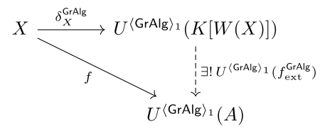 to commute, which says \(f^{\mathsf{GrAlg}}_{\mathrm{ext}}(\delta_{(x)}) = f(x)\) for all \(x \in X\). An element of \(\langle A \rangle_1\) is in particular an element of \(A\), so \(f\) is a function \(X \to U^{\mathsf{Alg}}_{}(A)\), and Theorem 1.5.17 gives the unique algebra homomorphism \(f^{\mathsf{Alg}}_{\mathrm{ext}}\colon K[W(X)] \to A\) with \(f^{\mathsf{Alg}}_{\mathrm{ext}}(\delta_{(x)}) = f(x)\). What is new is that it is graded. For \(u = (x_1) \frown \cdots \frown (x_n)\) of length \(n\) we have \(\delta_u = \delta_{(x_1)} \ast \cdots \ast \delta_{(x_n)}\), so \[f^{\mathsf{Alg}}_{\mathrm{ext}}(\delta_u) = f(x_1) \otimes \cdots \otimes f(x_n),\] a product of \(n\) elements of degree \(1\), which lies in \(A_n\) because \(A\) is a graded algebra. By linearity \(f^{\mathsf{Alg}}_{\mathrm{ext}}\) maps \(\langle K[W(X)] \rangle_n\) into \(A_n\), so it is an arrow of \(\mathsf{GrAlg}_K\), and the diagram commutes by construction. Uniqueness is inherited: a graded algebra homomorphism making the diagram commute is in particular an algebra homomorphism with \(\delta_{(x)} \mapsto f(x)\), hence equals \(f^{\mathsf{Alg}}_{\mathrm{ext}}\) (Exercise 1.6.9).
Example 1.6.20. Take \(X = \{x\}\), so \(K[W(X)] \cong K[x]\) (Example 1.5.19). Its grading is by polynomial degree: \(\langle K[x] \rangle_n = K\, x^n\). By Proposition 1.6.18, a graded algebra homomorphism \(K[x] \to A\) is the same as a choice of one element of \(\langle A \rangle_1\); an ungraded algebra homomorphism only needs an element of \(A\).
Example 1.6.21. For \(X = \{x, y\}\), write a word for its \(\delta\). The first few graded pieces of \(K[W(X)] = K\langle x, y \rangle\) are: \[\begin{array}{c|l|c} n & \text{basis of } \langle K\langle x, y \rangle \rangle_n & \dim \\ \hline 0 & \varepsilon & 1 \\ 1 & x,\ y & 2 \\ 2 & xx,\ xy,\ yx,\ yy & 4 \\ 3 & xxx,\ xxy,\ xyx,\ xyy,\ yxx,\ yxy,\ yyx,\ yyy & 8 \end{array}\] Each piece has dimension \(2^n\), as Proposition 1.6.15 predicts.
Discussion 1.6.22. We set out to make a set \(X\) into a vector space, and then into an algebra, in the best possible way. Each time, “best” turned out to mean initial in a comma category: \(F^{}_{\mathsf{Vect}}(X)\), \(F^{}_{\mathsf{Mon}}(X)\) and \(F^{}_{\mathsf{Alg}}(X)\) are defined by universal properties, and the constructions \(K^{(X)}\), \(W(X)\) and \(K[W(X)]\) are the evidence that such objects exist. Every proof followed the same pattern: a map out of a free object is determined by where the generators go.
Then something unexpected happened. The very same object, \(K[W(X)]\), turned out to be initial a second time, among graded algebras with \(X\) placed in degree \(1\). So “free” is not a property of an object alone: it depends on what we are forgetting. And we have only ever built free objects one set at a time. The next chapter asks how the free objects for all \(X\) fit together — the global form of these local constructions — and the answer is the notion of an adjunction.
One thread leads directly into what comes next. The degree-\(n\) part of \(K[W(X)]\) is the free vector space on \(X^n\). Once we have tensor products, \(K^{(X^n)}\) becomes the \(n\)-fold tensor power \(V^{\otimes n}\) of \(V = K^{(X)}\), and \(K[W(X)]\) becomes the tensor algebra \(T(V)\): the free graded algebra on a vector space placed in degree \(1\). So the free graded algebra on a set is itself a composite of free constructions, the free vector space followed by the tensor algebra, in exactly the sense of Lemma 1.5.15. Seeing these composites as composites of adjoint functors is the business of the next chapter.
Exercises
Exercise 1.6.1. Let \(\mathbb{N}\) also denote the category whose objects are the natural numbers and whose only arrows are identities. Show that giving a graded vector space is the same as giving a family \((V_0, V_1, V_2, \ldots)\) of vector spaces (a functor \(\mathbb{N} \to \mathsf{Vect}_K\)), and that a degree-preserving linear map is the same as a family of linear maps \(f_n\colon V_n \to W_n\), compatibly with composition. (In the language of later chapters, \(\mathsf{GrVect}_K\) is equivalent to the functor category \(\mathsf{Vect}_K^{\mathbb{N}}\).)
Exercise 1.6.2. Show that \(\mathsf{GrVect}_K\) is a category: composites of degree-preserving linear maps are degree-preserving, and identity maps are degree-preserving.
Exercise 1.6.3. Show that a grading \(V = \bigoplus_n V_n\) determines a complete system of orthogonal idempotents \(p_n\) (with \(p_n(v)\) the degree-\(n\) component of \(v\)), that such a system determines a grading \(V_n \coloneqq p_n(V)\), and that these two constructions are inverse to each other.
Exercise 1.6.4. Let \(A\) be an algebra whose underlying vector space is graded with \(A_n A_m \subseteq A_{n+m}\). Show that \(1_A \in A_0\).
Exercise 1.6.5. Let \(\beta\colon X \to Y\) be a bijection of sets. Show that \(\phi \mapsto \phi \circ \beta^{-1}\) is a linear isomorphism \(K^{(X)} \to K^{(Y)}\) sending \(\delta_x\) to \(\delta_{\beta(x)}\).
Exercise 1.6.6. Show that the two maps in the proof of Proposition 1.6.15 — restriction \(\langle K[W(X)] \rangle_n \to K^{(W_n(X))}\) and extension by zero \(K^{(W_n(X))} \to \langle K[W(X)] \rangle_n\) — are linear and mutually inverse.
Exercise 1.6.7. Show that if \(X\) has \(k\) elements, then \(\dim \langle K[W(X)] \rangle_n = k^n\).
Exercise 1.6.8. Show that for each \(n\), \(\langle - \rangle_n\colon \mathsf{GrAlg}_K \to \mathsf{Vect}_K\), sending \(A\) to \(\langle A \rangle_n\) and \(f\) to its restriction \(\langle A \rangle_n \to \langle B \rangle_n\), is a functor.
Exercise 1.6.9. Complete the sketch of Proposition 1.6.18: show that \(f^{\mathsf{GrAlg}}_{\mathrm{ext}}\) is well defined, an algebra homomorphism, graded, and unique.
Exercise 1.6.10. Show that a linear map \(f\colon V \to W\) between graded vector spaces is degree-preserving if and only if \(f \circ \langle - \rangle_n = \langle - \rangle_n \circ f\) for every \(n\).
Exercise 1.6.11. Let \(X\) have \(k\) elements. Record the dimensions of the graded pieces of \(K[W(X)]\) as the coefficients of a formal power series, \[\sum_{n=0}^{\infty} \dim\bigl(\langle K[W(X)] \rangle_n\bigr)\, t^n \in K[[t]],\] with \(K[[t]]\) and its convolution product as in Exercise 1.5.7, so that the coefficient of \(t^n\) in a product is the finite sum \(\sum_{i + j = n} a_i b_j\). Show that this series is \(1/(1 - kt)\), meaning that its product with \(1 - kt\) is \(1\).
Exercise 1.6.12. Regard \(K\) as a graded algebra with everything in degree \(0\). Show that the algebra homomorphism \(K[W(\{x\})] \to K\) with \(\delta_{(x)} \mapsto 1\) exists but is not graded. Which hypothesis of Proposition 1.6.18 fails?
Exercise 1.6.13. Show that the polynomial algebra \(K[x_1, \ldots, x_k]\) in \(k\) commuting variables is graded by total degree, and that its degree-\(n\) part has dimension \[\binom{n+k-1}{n}.\] Compare with \(k^n\) for the free algebra.
Exercise 1.6.14. Call a monoid \(M\) with a monoid homomorphism \(d\colon M \to \mathbb{N}\) a graded monoid. Show that graded monoids and degree-preserving homomorphisms form the slice of \(\mathsf{Mon}\) over \(\mathbb{N}\), and that \(K[M]\) is a graded algebra whose degree-\(n\) part is spanned by the \(\delta_m\) with \(d(m) = n\).
1.7 Notes and References
Notes and References 1.7.1.
Comma categories were introduced in Lawvere (1963), written \((S, T)\), which is the origin of the name. The arrow notation \(S \downarrow T\) is Mac Lane’s (Mac Lane 1998, sec. II.6). Slices and coslices are special cases (Exercise 1.2.2).
An initial object of \(X \downarrow U\) is what Mac Lane calls a universal arrow from \(X\) to \(U\) (Mac Lane 1998, sec. III.1). When one exists for every \(X\), they assemble into a left adjoint of \(U\); that is the global form of the constructions in this chapter.
The free vector space \(K^{(X)}\) follows Bourbaki’s notation for finitely supported families (Bourbaki 1989 Ch. II §1). It is also written \(K[X]\) or \(\bigoplus_{x \in X} K\).
The free monoid \(W(X)\) is the set of words over the alphabet \(X\), written \(X^\ast\) (Kleene star) in formal language theory. We avoid the star, which this book uses for duals.
The monoid algebra \(K[M]\) generalizes the group algebra \(K[G]\), the basic object of representation theory: a representation of \(G\) on a vector space \(V\) is the same as an algebra homomorphism \(K[G] \to \operatorname{End}(V)\), by Proposition 1.5.11 (a group homomorphism \(G \to \mathrm{GL}(V)\) is a monoid homomorphism into the monoid of \(\operatorname{End}(V)\)). Example 1.5.21 is \(K[C_2]\) for the group of order two. The free algebra \(K[W(X)]\) is usually written \(K\langle X \rangle\), the algebra of non-commutative polynomials; Chapter 2 relates it to the tensor algebra.
Notation. Hom-sets are written Kelly-style, \(\mathsf{C}(x, y)\) (Kelly 1982), rather than \(\mathop{\mathrm{Hom}}_{\mathsf{C}}(x, y)\). Free and forgetful functors carry their source as a superscript and target as a subscript (\(U^{\mathsf{Vect}}_{}\), \(F^{}_{\mathsf{Vect}}\)). The unique extension \(f^{\mathsf{Vect}}_{\mathrm{ext}}\) is elsewhere called the adjunct or transpose of \(f\), often written \(f^\sharp\) (e.g. Riehl 2016 Definition 4.1.1). Free objects are defined by their universal property, with constructions as existence proofs, which reverses the order of most texts.
Other treatments of the same material. Most texts do not spell out free constructions at all: the free vector space, free monoid and free algebra are stated and used, with the universal property mentioned in passing or left as an exercise. Among those that do, the framing of a free object as an initial object of \(X \downarrow U\) is Mac Lane’s universal arrow, done there in a page. Aluffi (2009, I.5 and II.5) is the nearest in spirit: free groups are defined as initial objects in a category of pairs \((G, j\colon A \to G)\) and only then constructed from words; he does groups and modules, not the monoid–algebra chain. Bergman (2015, Ch. 3–4) is the nearest in pace: a long, deliberate treatment of what “free” should mean before any construction, and the standard reference for universal-property-first exposition. Awodey (2010, sec. 1.7) treats the free monoid, with the word construction and its universal property, about as explicitly as §1.4 does. What none of them does is run the chain of this chapter, set to monoid to algebra, with each step defined by its universal property before it is built and the composite handled once (Lemma 1.5.15).
The route to the free algebra. Building the free algebra as the monoid algebra of the free monoid is Bourbaki’s (Bourbaki 1989 Ch. III §2, nos. 6–7, where the algebra of a monoid and the free algebra appear together) and is in Lang (2002, II.3, where the polynomial ring is the monoid algebra of a free commutative monoid). Both take the free monoid as obvious. The vector-space-first route, through the tensor algebra, is the one most texts take and is Chapter 2.
In the geometric algebra literature the construction is usually skipped entirely. Hestenes and Sobczyk (1984), Dorst et al. (2007) and Macdonald (2011) axiomatize the geometric product; Lounesto (2001), Garling (2011) and Lawson and Michelsohn (1989, Ch. I) define the Clifford algebra as a quotient of a tensor algebra taken as known, following Chevalley (1954). None starts from free constructions on a set. That is the gap this part of the book fills: the geometric algebra built from the ground up, with each universal object defined before it is constructed.